
- https://ai.googleblog.com/2019/06/applying-automl-to-transformer.html
- http://mat.uab.cat/~alseda/MasterOpt/
- http://ryanrossi.com/search.php
- https://iss.oden.utexas.edu/
- http://michele-ackerer.fr/algorithmic-graph-theory.htm
- http://www.columbia.edu/~mc2775/
- http://web.eecs.umich.edu/~dkoutra/tut/sdm17.html
- http://web.eecs.umich.edu/~dkoutra/tut/icdm18.html
- http://www.mlgworkshop.org/2019/
- https://www.computationalnetworkscience.org/
- http://ccni.hrl.com/
Learn about graph, graph representations, graph traversals and their running time.
Graph is mathematical abstract or generalization of the connection between entities. It is an important part of discrete mathematics -- graph theory.
And graph processing is widely applied in industry and science such as the network analysis, graph convolutional network (GCN), probabilistic graph model(PGM) and knowledge graph, which are introduced in other chapters.
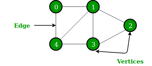
A graph
Graphs provide a powerful way to represent and exploit these connections. Graphs can be used to model such diverse areas as computer vision, natural language processing, and recommender systems. [^12]
The connections can be directed, weighted even probabilistic. It can be studied from the perspectives of matrix analysis and discrete mathematics.
All data in computer machine is digitalized bits. The primitive goal is to represent graph in computer as one data structure.
Definition: Let
$G=(V, E)$ be a graph with$V(G) = {1,\dots,n}$ and$E(G) = {e_1,\dots, e_m}$ . Suppose each edge of$G$ is assigned an orientation, which is arbitrary but fixed. The (vertex-edge)incidencematrix of$G$ , denoted by$Q(G)$ , is the$n \times m$ matrix defined as follows. The rows and the columns of$Q(G)$ are indexed by$V(G)$ and$E(G)$ , respectively. The$(i, j)$ -entry of$Q(G)$ is 0 if vertex$i$ and edge$e_j$ are not incident, and otherwise it is$\color{red}{\text{1 or −1}}$ according as$e_j$ originates or terminates at$i$ , respectively. We often denote$Q(G)$ simply by$Q$ . Whenever we mention$Q(G)$ it is assumed that the edges of$G$ are oriented.
| The adjacency matrix |
|---|
 |
Definition: Let
$G$ be a graph with$V(G) = {1,\dots,n}$ and$E(G) = {e_1,\dots, e_m}$ .Theadjacencymatrix of$G$ , denoted by$A(G)$ , is the$n\times n$ matrix defined as follows. The rows and the columns of$A(G)$ are indexed by$V(G)$ . If$i \not= j$ then the$(i, j)$ -entry of$A(G)$ is$0$ for vertices$i$ and$j$ nonadjacent, and the$(i, j)$ -entry is$\color{red}{\text{1}}$ for$i$ and$j$ adjacent. The$(i,i)$ -entry of$A(G)$ is 0 for$i = 1,\dots,n.$ We often denote$A(G)$ simply by$A$ .
Adjacency Matrixis also used to representweighted graphs. If the$(i, j)$ -entry of$A(G)$ is$w_{i, j}$ , i.e.$A[i][j] = w_{i, j}$ , then there is an edge from vertex$i$ to vertex$j$ with weight$w$ . TheAdjacency Matrixofweighted graphs$G$ is also calledweightmatrix of$G$ , denoted by$W(G)$ or simply by$W$ .
See Graph representations using set and hash at https://www.geeksforgeeks.org/graph-representations-using-set-hash/.
Definition: In graph theory, the degree (or valency) of a vertex of a graph is the number of edges incident to the vertex, with loops counted twice. From the wikipedia page at https://www.wikiwand.com/en/Degree_(graph_theory). The degree of a vertex
$v$ is denoted$\deg(v)$ or$\deg v$ .Degree matrix$D$ is a diagonal matrix such that$D_{i,i}=\sum_{j} w_{i,j}$ for theweighted graphwith$W=(w_{i,j})$ .
Definition: Let
$G$ be a graph with$V(G) = {1,\dots,n}$ and$E(G) = {e_1,\dots, e_m}$ .TheLaplacianmatrix of$G$ , denoted by$L(G)$ , is the$n\times n$ matrix defined as follows. The rows and the columns of$L(G)$ are indexed by$V(G)$ . If$i \not= j$ then the$(i, j)$ -entry of$L(G)$ is$0$ for vertices$i$ and$j$ nonadjacent, and the$(i, j)$ -entry is$\color{red}{\text{ −1}}$ for$i$ and$j$ adjacent. The$(i,i)$ -entry of$L(G)$ is$\color{red}{d_i}$ , the degree of the vertex$i$ , for$i = 1,\dots,n.$ In other words, the$(i,i)$ -entry of$L(G)$ , ${L(G)}{i,j}$, is defined by $${L(G)}{i,j} = D - A = \begin{cases} \deg(V_i) & \text{if$i=j$ ,}\ -1 & \text{if$i\not= j$ and$V_i$ and$V_j$ is adjacent,} \ 0 & \text{otherwise.}\end{cases}$$ Laplacian matrix of a graph$G$ withweighted matrix$W$ is${L^{W}=D-W}$ , where$D$ is the degree matrix of$G$ . We often denote$L(G)$ simply by$L$ .
Definition: A directed graph (or
digraph) is a set of vertices and a collection of directed edges that each connects an ordered pair of vertices. We say that a directed edge points from the first vertex in the pair and points to the second vertex in the pair. We use the names 0 through V-1 for the vertices in a V-vertex graph. Via https://algs4.cs.princeton.edu/42digraph/.
Adjacency List is an array of lists. An entry array[i] represents the list of vertices adjacent to the ith vertex. This representation can also be used to represent a weighted graph. The weights of edges can be represented as lists of pairs.
See more representation of graph in computer in https://www.geeksforgeeks.org/graph-data-structure-and-algorithms/.
Although the adjacency-list representation is asymptotically at least as efficient as the adjacency-matrix representation, the simplicity of an adjacency matrix may make it preferable when graphs are reasonably small. Moreover, if the graph is unweighted, there is an additional advantage in storage for the adjacency-matrix representation.

| Cayley graph of F2 in Wikimedia | Moreno Sociogram 1st Grade |
|---|---|
 |
 |
- http://mathworld.wolfram.com/Graph.html
- https://www.wikiwand.com/en/Graph_theory
- https://www.wikiwand.com/en/Gallery_of_named_graphs
- https://www.wikiwand.com/en/Laplacian_matrix
- https://www.wikiwand.com/en/Cayley_graph
- https://www.wikiwand.com/en/Network_science
- https://www.wikiwand.com/en/Directed_graph
- https://www.wikiwand.com/en/Directed_acyclic_graph
It seems that graph theory is partially the application of nonnegative matrix theory. Graph Algorithms in the Language of Linear Algebra shows how to leverage existing parallel matrix computation techniques and the large amount of software infrastructure that exists for these computations to implement efficient and scalable parallel graph algorithms. The benefits of this approach are reduced algorithmic complexity, ease of implementation, and improved performance.
| Matrix Theory | Graph Theory | ----- | --- |
|---|---|---|---|
| Matrix Addition | ? | Spectral Theory | ? |
| Matrix Power | ? | Jordan Form | ? |
| Matrix Multiplication | ? | Rank | ? |
| Basis | ? | Spectra | ? |
Definition A
walkin a digraph is an alternating sequence of vertices and edges that begins with a vertex, ends with a vertex, and such that for every edge$\left<u\to v\right>$ in the walk, vertex$u$ is the element just before the edge, and vertex$v$ is the next element after the edge.
A payoff of this representation is that we can use matrix powers to count numbers
of walks between vertices. The adjacent matrix
Definition The length-k walk counting matrix for an n-vertex graph
The length-k counting matrix of a digraph
$G$ is${A(G)}^k$ , for all$k\in\mathbb{N}$ .
Definition A walk in an undirected graph is a sequence of vertices, where each successive pair of vertices are adjacent; informally, we can also think of a walk as a sequence of edges. A walk is called a path if it visits each vertex at most once. For any two vertices
$u$ and$v$ in a graph$G$ , we say that$v$ is reachable from$u$ if$G$ contains a walk (and therefore a path) between$u$ and$v$ . An undirected graph is connected if every vertex is reachable from every other vertex. A cycle is a path that starts and ends at the same vertex and has at least one edge.
We will limit our attention to undirected graphs and view them as a discrete analog of manifolds. We define the vertex set vertex weights as the function edge weights as weighted undirected graph.
If
- Function on vertices(vertex field):
$s : V \to \mathbb R$ ; - Edge flows(edge field ):
$X:V\times V\to \mathbb R$ , where$X(i, j)=0,$ if$(i, j)\not\in E$ and$X(i, j)=-X(j,i)$ for all$(i, j)$ . - Triangular flows:
$\Phi: V\times V\times V\to\mathbb R$ where$\Phi(i, j ,k)=0$ if$(i, j, k)\not\in T$ and$\Phi(i, j, k)=\Phi(k, i, j)=\Phi(j, k, i)=-\Phi(j, i, k)=-\Phi(i, k, j)=-\Phi(k,j,i)$ for all$i, j, k$ .
| Operators | Definition |
|---|---|
| Graph gradient: grad | |
| Graph curl: curl | |
| Graph divergence: div | |
| Graph Laplacian | |
| Graph Helmholtzian |
(Helmholtz decomposition):$G = (V; E)$ is undirected, unweighted graph.
$\Delta_1$ is its Helmholtzian. The space of edge flows admits orthogonal decomposition:$$L^2(E)=im(grad)\oplus ker(\Delta_1)\oplus im(curl^{\ast}).$$ Furthermore,$ker(\Delta_1) = ker(curl) \cap ker(div)$ .
- http://www.mit.edu/~parrilo/
- https://www.stat.uchicago.edu/~lekheng/
- https://en.wikipedia.org/wiki/Graph_operations
- https://igraph.org/
- https://phorgyphynance.wordpress.com/2011/12/04/network-theory-and-discrete-calculus-graph-divergence-and-graph-laplacian/
- https://phorgyphynance.wordpress.com/network-theory-and-discrete-calculus/
- https://math.stackexchange.com/questions/1960191/function-and-divergence-on-a-graph
In graph theory, the shortest path problem is the problem of finding a path between two vertices (or nodes) in a graph such that the sum of the weights of its constituent edges is minimized.
Given the start node and end node, it is supposed to identify whether there is a path and find the shortest path(s) among all these possible paths.
The distance between the node
Because it is unknown whether there is a path between the given nodes, it is necessary to take the first brave walk into a neighbor of the start node
Breadth first search explores the space level by level only when there are no more states to be explored at a given level does the algorithm move on to the next level. We implement BFS using lists open and closed to keep track of progress through the state space. In the order list, the elements will be those who have been generated but whose children have not been examined. The closed list records the states that have been examined and whose children have been generated. The order of removing the states from the open list will be the order of searching. The open is maintained as a queue on the first in first out data structure. States are added to the right of the list and removed from the left.
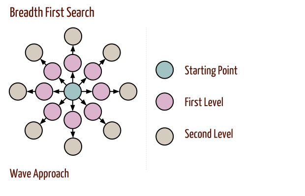
After initialization, each vertex is enqueued at most once and hence dequeued at most once.
The operations of enqueuing and dequeuing take
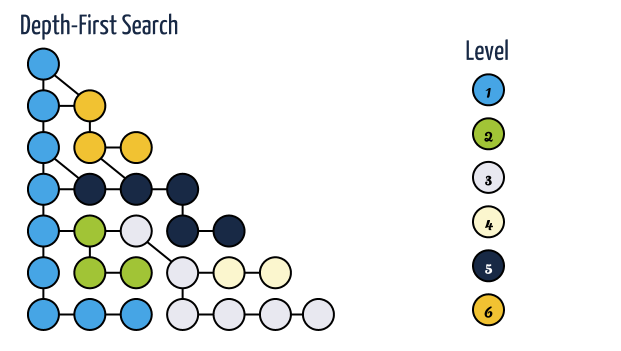
In depth first search, when a state is examined all of its children and their descendants are examined before any of its siblings. Depth first search goes deeper into the search space whenever this is possible, only when no further descendants of a state can be found, are its siblings considered.
A depth first traversal takes O(N*E) time for adjacency list representation and
- https://brilliant.org/wiki/depth-first-search-dfs/
- Breadth First Search (BFS) and Depth First Search (DFS) Algorithms
As introduced in wikipedia,
In computer science,
$A^{\ast}$ (pronounced "A star") is a computer algorithm that is widely used in path finding and graph traversal, which is the process of finding a path between multiple points, called "nodes". It enjoys widespread use due to its performance and accuracy. However, in practical travel-routing systems, it is generally outperformed by algorithms which can pre-process the graph to attain better performance, although other work has found$A^{\ast}$ to be superior to other approaches.
First we learn the Dijkstra's algorithm. Dijkstra's algorithm is an algorithm for finding the shortest paths between nodes in a graph, which may represent, for example, road networks. It was conceived by computer scientist Edsger W. Dijkstra in 1956 and published three years later.
For example, we want to find the shortest path between a and b in the following graph. The distance of every pair is given.
- the distance to its neighbors is computed:
| a(0) | 2 | 3 | 6 |
|---|---|---|---|
| 0 | 7 | 9 | 14 |
- as the first step, compute the distance to all neighbors:
| 2 | 3 | 4 | 3 | 4 | 6 |
|---|---|---|---|---|---|
| 0 | 10 | 15 | 0 | 11 | 2 |
Now we have 2 choices from 1 to 3: (1)
From 1 to 4: (1)
From 1 to 6: (1)
- distance to neighbor:
| 4 | b | 6 | b |
|---|---|---|---|
| 0 | 6 | 0 | 9 |
| Dijkstra algorithm |
|---|
 |
- https://www.wikiwand.com/en/Dijkstra%27s_algorithm
- https://www.geeksforgeeks.org/dijkstras-shortest-path-algorithm-greedy-algo-7/
- https://www.wikiwand.com/en/Shortest_path_problem
- https://www.cnblogs.com/chxer/p/4542068.html
- Introduction to $A^{\ast}$: From Amit’s Thoughts on Pathfinding
- Graph Search Algorithms by Steve Mussmann and Abi See
See the page at Wikipedia $A^{\ast}$ search algorithm
Perhaps even more important is the duality that exists with the fundamental operation of linear algebra (vector matrix multiply) and a breadth-first search (BFS) step performed on G from a starting vertex s: $$ BFS(G, s) \iff A^T v, v(s)=1. $$
This duality allows graph algorithms to be simply recast as a sequence of linear algebraic operations. Many additional relations exist between fundamental linear algebraic operations and fundamental graph operations
- Graph Algorithms in the Language of Linear Algebra
- Mathematics of Big Data: Spreadsheets, Databases, Matrices, and Graphs
- Dual Adjacency Matrix: Exploring Link Groups in Dense Networks by K. Dinkla N. Henry Riche M.A. Westenberg
- On the p-Rank of the Adjacency Matrices of Strongly Regular Graphs
- Matrix techniques for strongly regular graphs and related geometries
Directed acyclic graph (DAG) is the directed graph without any cycles. It is used widely in scheduling, distributed computation.
Definition The acyclic graph is called
forest. A connected acyclic graph is called atree.
A graph
Topological sorting for Directed Acyclic Graph (DAG) is a linear ordering of vertices such that for every directed edge
Graph theory applied in the study of molecular structures represents an interdisciplinary science, called chemical graph theory or molecular topology.
A chemical graph is a model of a chemical system, used to characterize the
interactions among its components: atoms, bonds, groups of atoms or molecules. A structural formula
of a chemical compound can be represented by a molecular graph, its
vertices being atoms and edges corresponding to covalent bonds.
Usually hydrogen atoms are not depicted in which case we speak of hydrogen depleted molecular graphs.
In a multigraph two points may be joined by more than one line.
If multibonds are taken into account, a variant of adjacency matrix
Distance Matrix
M. V. Diudea, I. Gutman and L. Jantschi in Molecular Topology claims that
A single number, representing a chemical structure, in graph-theoretical terms, is called a
topological descriptor. Being a structural invariant it does not depend on the labeling or the pictorial representation of a graph. Despite the considerable loss of information by the projection in a single number of a structure, such descriptors found broad applications in the correlation and prediction of several molecular properties1,2 and also in tests of similarity and isomorphism.
The simplest TI is the half sum of entries in the adjacency matrix
The Indices of Platt, F, Gordon-Scantlebury, N2, and Bertz, B1:
$$F={\sum}{i}\sum{j}{[EA]}{ij}=2\sum{i}C_{2}^{\delta_i}=2 N2=2 B1$$
where
First TIs based on adjacency matrix (i.e., based on connectivity) were introduced
by the Group from Zagreb:
$$
M_1=\sum_{i}\delta_i^2, \
M_2=\sum_{(i,j)\in E(G)}\delta_i\delta_j
$$
where
The Randic Index,
It can extended the summation over all paths of
length
Wiener-Type Indices
In acyclic structures, the Wiener index, W and its extension, the hyper-Wiener
index, WW can be defined as
$$
W=W(G)={\sum}e N{i,e}N_{e,j} \
WW=WW(G)={\sum}e N{i,p}N_{p, j}
$$
where
INDICES BASED ON RECIPROCAL MATRICES
INDICES BASED ON COMBINATION OF MATRICES
INDICES BASED ON EIGENVALUES AND EIGENVECTORS
Topological descriptors Topological index
- Virtual Computational Chemistry Laboratory
- Molecular Topology File
- MATHEMATICAL CHALLENGES FROM THEORETICAL/COMPUTATIONAL CHEMISTRY
- The Universe of Chemical Mathematics and the Worlds of Mathematical Chemistry
- http://www.estradalab.org/research-description-three/
- Mathematical Issues for Chemists
- https://www.wikiwand.com/en/Mathematical_chemistry
- http://match.pmf.kg.ac.rs/
- https://crystalmathlabs.com/tracker/
Definition: Separators A subsect of vertices
The fundamental problem that is trying to solve is that of splitting a large irregular graphs into
${k}$ parts. This problem has applications in many different areas including, parallel/distributed computing (load balancing of computations), scientific computing (fill-reducing matrix re-orderings), EDA algorithms for VLSI CAD (placement), data mining (clustering), social network analysis (community discovery), pattern recognition, relationship network analysis, etc. The partitioning is usually done so that it satisfies certain constraints and optimizes certain objectives. The most common constraint is that of producing equal-size partitions, whereas the most common objective is that of minimizing the number of cut edges (i.e., the edges that straddle partition boundaries). However, in many cases, different application areas tend to require their own type of constraints and objectives; thus, making the problem all that more interesting and challenging!The research in the lab is focusing on a class of algorithms that have come to be known as multilevel graph partitioning algorithms. These algorithms solve the problem by following an approximate-and-solve paradigm, which is very effective for this as well as other (combinatorial) optimization problems.
- Graph Partitioning
- Gary L. Miller's Publications on Graph Separartor
- Points, Spheres, and Separators: A Unified Geometric Approach to Graph Partitioning
Let
Definition A

A Spectral Analysis of Moore Graphs
As the title suggests, Spectral Graph Theory is about the eigenvalues and eigenvectors of matrices associated
with graphs, and their applications.
---|---
---|---
Adjacency matrix|
For the symmetric matrix
Let
$G = (V;E)$ be a graph, and let$\lambda=(\lambda_1, \cdots, \lambda_n)^T$ be the eigenvalues of its Laplacian matrix. Then,$\lambda_2>0$ if and only if G is connected.
There are many iterative computational methods to approximate the eigenvalues of the graph-related matrices.
Raluca Tanase and Remus Radu, in The Mathematics of Web Search, asserted that
The usefulness of a search engine depends on the relevance of the result set it gives back. There may of course be millions of web pages that include a particular word or phrase; however some of them will be more relevant, popular, or authoritative than others. A user does not have the ability or patience to scan through all pages that contain the given query words. One expects the relevant pages to be displayed within the top 20-30 pages returned by the search engine.
Modern search engines employ methods of ranking the results to provide the "best" results first that are more elaborate than just plain text ranking. One of the most known and influential algorithms for computing the relevance of web pages is the Page Rank algorithm used by the Google search engine. It was invented by Larry Page and Sergey Brin while they were graduate students at Stanford, and it became a Google trademark in 1998. The idea that Page Rank brought up was that, the importance of any web page can be judged by looking at the pages that link to it. If we create a web page i and include a hyperlink to the web page j, this means that we consider j important and relevant for our topic. If there are a lot of pages that link to j, this means that the common belief is that page j is important. If on the other hand, j has only one backlink, but that comes from an authoritative site k, (like www.google.com, www.cnn.com, www.cornell.edu) we say that k transfers its authority to j; in other words, k asserts that j is important. Whether we talk about popularity or authority, we can iteratively assign a rank to each web page, based on the ranks of the pages that point to it.
PageRank is the first importance measure of webpage in large scale application. And this is content-free so that it does not take the relevance of webpages into consideration.

Here's how the PageRank is determined. Suppose that page
Note that the importance ranking of
The condition above defining the PageRank
$$ I = {\bf H}I $$ In other words, the vector I is an eigenvector of the matrix H with eigenvalue 1. We also call this a stationary vector of H.
It is not very simple and easy to compute the eigenvalue vectors of large scale matrix.
If we denote by $\bf 1$the
$$ {\bf G}=\alpha{\bf S}+ (1-\alpha)\frac{1}{n}{\bf 1} $$ Notice now that G is stochastic as it is a combination of stochastic matrices. Furthermore, all the entries of G are positive, which implies that G is both primitive and irreducible. Therefore, G has a unique stationary vector I that may be found using the power method.
- Page rank@wikiwand
- The Anatomy of a Large-Scale Hypertextual Web Search Engine by Sergey Brin and Lawrence Page
- Learning Supervised PageRank with Gradient-Based and Gradient-Free Optimization Methods
- Lecture #3: PageRank Algorithm - The Mathematics of Google Search
- HITS Algorithm - Hubs and Authorities on the Internet
- http://langvillea.people.cofc.edu/
- Google PageRank: The Mathematics of Google
- How Google Finds Your Needle in the Web's Haystack
- Dynamic PageRank
- https://www.cnblogs.com/chenying99/archive/2012/06/07/2540013.html
- https://blog.csdn.net/aspirinvagrant/article/details/40924539
Spectral method is the kernel tricks applied to locality preserving projections as to reduce the dimension, which is as the data preprocessing for clustering.
In multivariate statistics and the clustering of data, spectral clustering techniques make use of the spectrum (eigenvalues) of the similarity matrix of the data to perform dimensionality reduction before clustering in fewer dimensions.
The similarity matrix is provided as an input and consists of a quantitative assessment of the relative similarity of each pair of points in the data set.
Similarity matrix is to measure the similarity between the input features ${\mathbf{x}i}{i=1}^{n}\subset\mathbb{R}^{p}$. For example, we can use Gaussian kernel function $$ f(\mathbf{x_i},\mathbf{x}j)=exp(-\frac{{|\mathbf{x_i}-\mathbf{x}j|}2^2}{2\sigma^2}) $$ to measure the similarity of inputs. The element of similarity matrix $S$ is $S{i, j} = exp(-\frac{{| \mathbf{x_i} -\mathbf{x}j|}2^2}{2\sigma^2})$. Thus $S$ is symmetrical, i.e. $S{i, j}=S{j, i}$ for $i,j\in{1,2,\dots, n}$. If the sample size $n\gg p$, the storage of similarity matrix is much larger than the original input ${\mathbf{x}i }{i=1}^{n}$, when we would only preserve the entries above some values. The Laplacian matrix is defined by $L=D-S$ where $D = Diag{D_1, D_2, \dots, D_n}$ and $D{i} = \sum{j=1}^{n} S_{i,j} = \sum_{j=1}^{n} exp(-\frac{{|\mathbf{x_i} - \mathbf{x}_j|}_2^2}{2\sigma^2})$.
Then we can apply principal component analysis to the Laplacian matrix
- https://zhuanlan.zhihu.com/p/34848710
- On Spectral Clustering: Analysis and an algorithm at http://papers.nips.cc/paper/2092-on-spectral-clustering-analysis-and-an-algorithm.pdf
- A Tutorial on Spectral Clustering at https://www.cs.cmu.edu/~aarti/Class/10701/readings/Luxburg06_TR.pdf.
- 谱聚类 https://www.cnblogs.com/pinard/p/6221564.html.
- Spectral Clustering http://www.datasciencelab.cn/clustering/spectral.
- https://en.wikipedia.org/wiki/Category:Graph_algorithms
- The course Spectral Graph Theory, Fall 2015 at http://www.cs.yale.edu/homes/spielman/561/.
- IE532. Analysis of Network Data, Sewoong Oh, University of Illinois Urbana-Champaign.
- https://skymind.ai/wiki/graph-analysis
Like kernels in kernel methods, graph kernel is used as functions measuring the similarity of pairs of graphs. They allow kernelized learning algorithms such as support vector machines to work directly on graphs, without having to do feature extraction to transform them to fixed-length, real-valued feature vectors.
Definition : Find a mapping isomorphic.
No polynomial-time algorithm is known for graph isomorphism. Graph kernel are convolution kernels on pairs of graphs. A graph kernel makes the whole family kernel methods applicable to graphs.
Von Neumann diffusion is defined as
Exponential diffusion is defined as Katz method is defined as the truncation of Von Neumann diffusion
- https://www.wikiwand.com/en/Graph_product
- https://www.wikiwand.com/en/Graph_kernel
- Graph Kernels
- GRAPH KERNELS by Karsten M. Borgwardt
- List of graph kernels
- Deep Graph Kernel
- Topological Graph Kernel on Multiple Thresholded Functional Connectivity Networks for Mild Cognitive Impairment Classification
- Awesome Graph Embedding
- Document Analysis with Transducers
Dirichlet energy functional is defined as
The above algorithms are unsupervised algorithms so what is the supervised algorithms in graph data sets? Do prediction algorithms such as classification and regression matter?
It is to answer the question how to characterize a network in the term of some summary statistic. The following distribution may be the key:
- the distribution of the degree;
- the distribution of the eigenvalue of the Laplacian matrix;
- random matrix and dynamical network.
A particle moves around the vertex-set
- Under what conditions is the walk recurrent, in that it returns (almost surely) to its starting point?
- How does the distance between S0 and Sn behave as
$n\to\infty$ ?
Computational graphs are a nice way to think about mathematical expressions, where the mathematical expression will be in the decomposed form and in topological order.

To create a computational graph, we make each of these operations, along with the input variables, into nodes. When one node’s value is the input to another node, an arrow goes from one to another. These sorts of graphs come up all the time in computer science, especially in talking about functional programs. They are very closely related to the notions of dependency graphs and call graphs. They’re also the core abstraction behind the popular deep learning framework TensorFlow.
Computational graph is an convenient representation of the work flow or process pipeline, which describes the dependence/composite relationship of every variable.
Additionally, each composite relationship is specified.
Decision tree looks like simple graph without loops, where only the leaf nodes specify the output values and the middle nodes specify their test or computation.
- https://colah.github.io/posts/2015-08-Backprop/
- Visualization of Computational Graph@chainer.org
- Efficiently performs automatic differentiation on arbitrary functions.
- 计算图反向传播的原理及实现
- 运用计算图搭建 LR、NN、Wide & Deep、FM、FFM 和 DeepFM
- A Computational Network
- http://ww3.algorithmdesign.net/sample/ch07-weights.pdf
- https://www.geeksforgeeks.org/graph-data-structure-and-algorithms/
- https://www.geeksforgeeks.org/graph-types-and-applications/
- https://algs4.cs.princeton.edu/40graphs/
- http://networkscience.cn/
- http://www.ericweisstein.com/encyclopedias/books/GraphTheory.html
- http://mathworld.wolfram.com/CayleyGraph.html
- http://yaoyao.codes/algorithm/2018/06/11/laplacian-matrix
- The book Graphs and Matrices https://www.springer.com/us/book/9781848829800
- The book Random Graph https://www.math.cmu.edu/~af1p/BOOK.pdf
- The book Graph Signal Processing: Overview, Challenges and Application
- http://www.andres.sc/graph.html
- https://github.com/sungyongs/graph-based-nn
- Probabilistische Graphische Modelle
- NetworkX : a Python package for the creation, manipulation, and study of the structure, dynamics, and functions of complex networks
- The Neo4j Graph Algorithms User Guide v3.5
- Matlab tools for working with simple graphs
- GSoC 2018 - Parallel Implementations of Graph Analysis Algorithms
- Graph theory (network) library for visualization and analysis
- graph-tool | Efficient network analysis
- JGraphT: a Java library of graph theory data structures and algorithms
- Stanford Network Analysis Project