Pytorch-Vision-Transformer

Vision Transformer implemented from scratch in Pytorch From Attention to ‘Attention is All You Need’ The attention mechanism was first proposed for language translation tasks by Yoshua Bengio’s lab in a paper at ICLR 2015 [1]. It was initially called an ‘alignment’ model in that the attention scores measured the alignment of two words, with the alignment being high if the dot product of the query and key vectors was large. However, in this paper, the key and query vectors were not computed as we explained in the previous post but were rather the outputs and hidden states of a recurrent block. In hindsight, we know that the recurrent parts of the architecture hamstrung the performance of the model Even so, the proposed model was already comparable to the state of the art on English to French translation task at that time.

In subsequent years and months, several variants of this mechanism were proposed such that RNNs, LSTMs or GRUs were always a part of the model. However, in 2017, Vaswani et. al. from Google Brain proposed to completely remove all recurrent connections from the model such that one ends up with a pure attention based model. Thus, one of the most famous papers of the last decade was born and aptly named: “Attention is All You Need”

Figure 1. The original transformer model proposed by Vaswani et. al. The left gray box represents an encoder layer while the right box represents a decoder layer. We have not introduced all the components of this architecture yet, but please note that the most critical component is the multi-headed self-attention module.

The architecture proposed in this paper transforms an input sequence into an output sequence. Hence, the name ‘transformer’. Figure 1 shows the transformer architecture. The architecture consists of an encoder (left of figure 1) and a decoder (right of figure 1). The encoder uses MHSA to transform the input sequence into a hidden representation, while the decoder takes the hidden representation from the encoder and predicts the output. There are a few elements from the figure that we have not introduced yet, but the basic structure should look familiar. Within the gray encoder and decoder blocks, notice additional residual connections on top of the MHSA layers, so that the gradient can propagate easily while training. Thus, even though the attention mechanism is multiplicative (somewhat like vanilla RNNs), the residual connections help with training and transformers do not suffer from exploding and vanishing gradients like vanilla RNNs.

The reasons for the success of transformers The most important result from this paper was that transformers not only performed better than other models but also about an order of magnitude faster to train and utilized the computational resources more efficiently than competing methods like additive attention. To summarize, the key reasons for the success of transformers are:

1.Multi Headed Self attention layers (of course) 2.Use of Layer normalization rather than batch normalization 3.Scaling the attention matrix to improve gradient flow. 4.Residual connections in the ender and decoder layers, and 5.Presence of cross attention between encoder and decoder layers.

The Vision Transformer And Its Components Figure 2. The architecture of the vision transformer model proposed by Dosovitskiy et. al. The model uses only the encoder part of the full transformer architecture proposed by Vaswani et. al. An image is split up into patches that are linearly embedded. A classification token, just like in the BERT model, is concatenated, and position embeddings are added. The resulting sequence is fed into the transformer encoder. Finally, a small MLP head on top of the classification token patch is used to read out the classification output.The architecture of the vision transformer model is shown in figure 2. The caption of the figure contains several terms like class token, and position embedding, which are also present in figure 1.

Patch Embeddings Figure 3. How to create patch embeddings from an image. Transformer models process inputs as words or tokens. If we want to apply transformers to image recognition, the first question to ask is ‘what is the equivalent of words in images?’ There are several choices, such as treating each pixel as a word. However, we note that the computational complexity of calculating the attention matrix is N2 where N is the sequence length. If we treat each pixel as a separate word, then assuming a relatively small image size of 100×100, the attention matrix will be of size 10000×10000. This is obviously unmanageable even for the largest GPUs. Figure 4. An input image of size 224×224 with a patch size of 16×16 and an embedding dimension of 768 results in a learnt patch representation of size 196×768. A more moderate choice is to treat a patch of some size, say 16×16, as one word. Thus, as shown in figure 3, the RGB image of size WxHx3 is divided up into patches, each of size wxhx3. Each patch is flattened and passed through a dense layer without activation, called an embedding layer. The same weights are reused for all patches of the image. The embedding layer transforms the patch into a hidden, learned representation of dimension din. Finally, note that before creating the patches, the input image is preprocessed by subtracting the mean and dividing by the standard deviation, just like for any other image classification model.

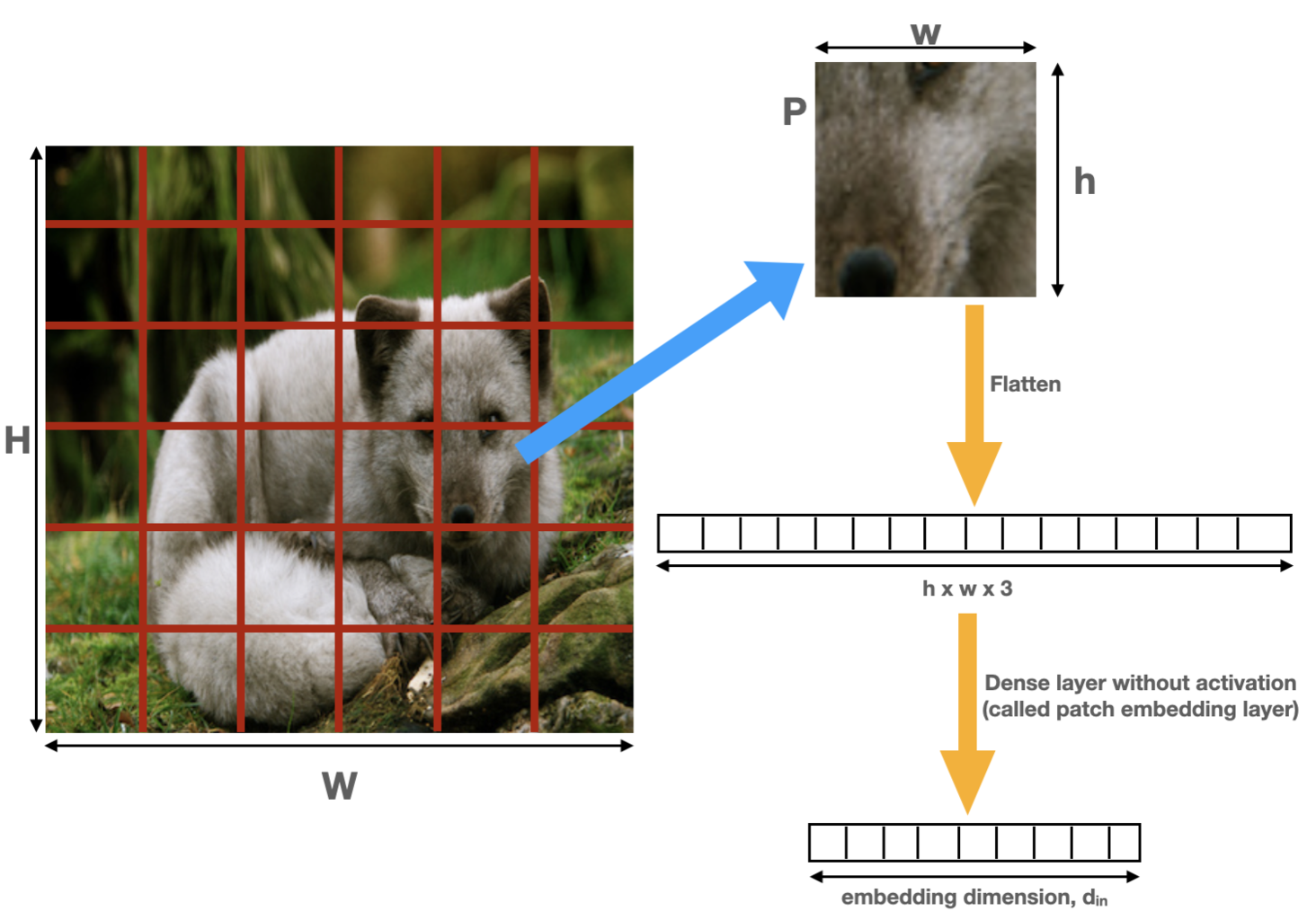
Let us take the example of the imagenet dataset. As shown in figure 4, an image of size 224×224 pixels (W=H=224) is divided up into patches of size 16×16 (w=h=16). Thus, 14×14 (since 224/16=14) or a total of 196 patches are created from one image. In terms of tensor sizes, assuming a batch size of 1, the input image is of size [1, 3, 224, 224] while after patch embedding, the tensor has size [1, 196, din]. For example, din = 768 in the base vision transformer model.

Classification Token Figure 5. Concatenating a classification token (patch) at the beginning of the image patch sequence. This token is used to read out the classification output from the model. Computer vision has enjoyed the benefits of transfer learning for a long time. However, even as late as 2018, NLP models could not effectively be pre-trained on some datasets and fine-tuned on another for a different task. This changed with the introduction of Bidirectional Encoder Representations from Transformers or BERT. BERT framed the pre-training task as a classification problem. To let the transformer model perform classification, an extra token called the class token was used.

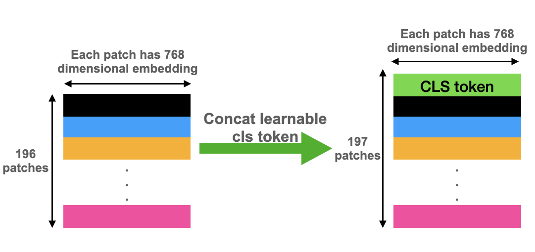
Vision transformers adopt this concept from BERT. The idea is to concatenate a learnable patch to the beginning of the patch sequence, as shown in figure 5. This patch is used read out the classification output at the end of the model, as we will explain in section 2.6. In terms of tensor sizes, continuing with our example of an image, the size before concatenation was [1,196,768]. After concatenating a learnable parameter (nn.Parameter in PyTorch) called class token, the resulting tensor has a size [1,197,768]. This is the size of the input tensor to the transformer model. Thus, recalling the notation from the first part of this series, N=197 and din=768.

Position Embedding Figure 6. Position embedding.

There are many kinds of position embeddings in the NLP literature such as the sine/cosine embeddings and learnable embeddings. Vision transformers work about the same with either of these types. So, we will work with learnable position embeddings.

As shown in figure 6, a position embedding is just a learnable parameter. Continuing with our example of images of size 224×224, recall that after concatenating the classification token, the tensor has size [1, 197, 768]. We instantiate the position embedding parameter to be of the same size and add the patches and position embedding element-wise. The resulting sequence of vectors is then fed into the transformer model.

Layer Normalization Figure 7. Schematic explanation of layer normalization Layer normalization, first proposed by the legendary Professor Geoffrey Hinton’s lab, is a slightly different version of batch normalization. We are all familiar with batch norm in the context of computer vision. However, batch norm cannot be directly applied to recurrent architectures. Moreover, since the mean (μ) and standard deviation (σ) statistics in batch norm are calculated for a mini-batch, the results are dependent on the batch size. As shown in figure 7, layer normalization overcomes this problem by calculating the statistics for the neurons in a layer rather than across the mini batch. Thus, each sample in the mini batch gets a different μ and σ, but the mean and std deviation are the same for all neurons in a layer.

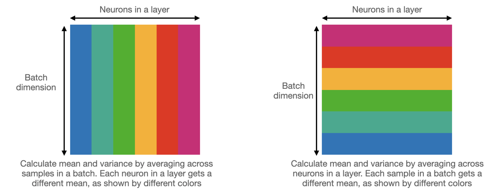
The thing to note is that for typical model sizes, layer norm is slower than batch norm. Thus, some architectures like DEST (which are designed for speed, but we will not introduce them here), use engineering tricks to use batch norm while keeping the training stable. However, for most widely used vision transformers, layer norm is used and is quite critical for their performance.

Multi-Layer Perceptron

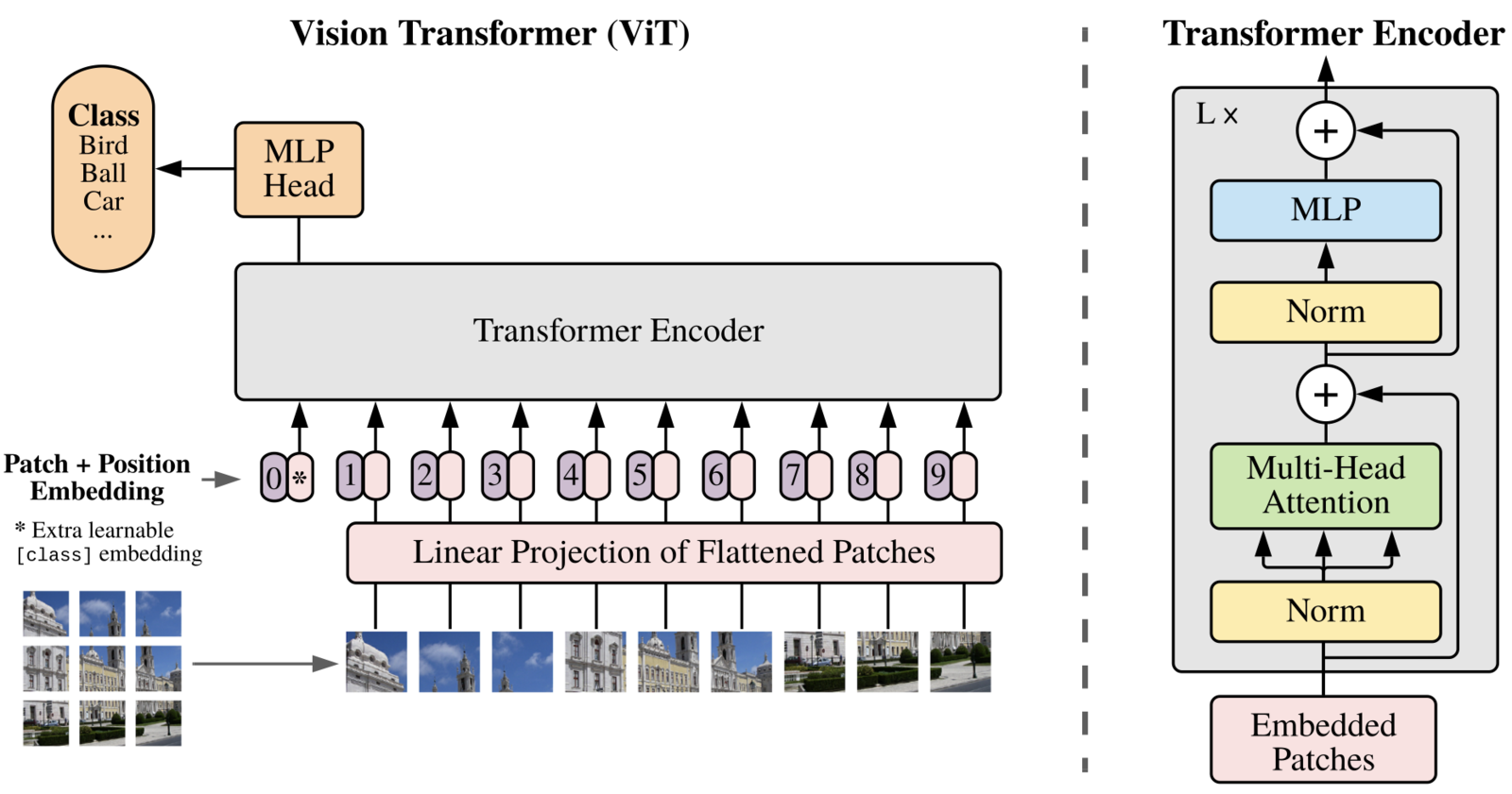
As you can see from figure 1 and 2, the encoder layer of the transformer architecture has a feed-forward or MLP module. This is a short sequential module consisting of:

1.A linear layer that projects the output of the MHSA layer into higher dimensions (dmlp>din) 2.An activation layer with GELU activation (GELU(x) = xɸ(x), where ɸ(x) is the cumulative distribution function of the standard gaussian distribution) 3.A dropout layer to prevent overfitting 4.A linear layer to the projects the output back to the same size as the output of the MHSA layer. 5.Another dropout layer to prevent overfitting.

Classification Head We remarked in the above section on ‘classification token’ that a learnable parameter called a classification token is concatenated to the patch embeddings. This token becomes a part of the vector sequence fed into the transformer model and evolves with self-attention. Finally, we attach a small MLP classification head on top of this module and read the classification results from it. This is just a vanilla dense layer with the number of neurons equal to the number of classes in the dataset. So, for example, continuing with our example of din=768, for imagenet dataset, this layer will take in a vector of size 768 and output 1000 class probabilities.

Note that once we have obtained the classification probabilities from the MLP head on top of the classification token, the outputs from all other patches is IGNORED! This seems quite unintuitive and one may wonder why the classification token is required at all. After all, can’t we average the outputs from all the other tokens and train an MLP on top of that, much like what we do with ResNets? Yes, it is quite possible to do so and it works just as well as the classification token approach. Just note that a different, lower learning rate is required to get this to work.

Putting everything together

We now have all the components required to implement a vision transformer. Let us summarize all the components of the ViT architecture:

1.The input images to a ViT model are first pre-processed with mean and standard deviation scaling, just like any other vision model. 2.The images in a batch are then split up into patches 3.The patches are linearly embedded with a learnable layer as explained in section 2.1 4.A learnable parameter called classification token is concatenated to the patch embeddings, as explained in section 2.2. 5.Another learnable parameter called position embedding is added element wise to the patch embeddings (with cls token). 6.The resulting sequence of vectors is fed into a transformer encoder layer. There are L such layers (typically L=12 or 24). The output of each encoder layer has the same shape as the input. 7.Every layer of the encoder consists of: A layer normalization module Multi headed self attention (MHSA) module, explained in previous post Residual connection from the input of the layer to the output of the MHSA module Another layer normalization, and finally The Multi-layer perceptron module explained in the subsection 2.5 1.Finally, a classification head is attached to the top of the output corresponding to the class token which outputs the probabilities for each class.

Implementing The Vision Transformer in PyTorch Implementing MHSA module

Since we had already introduced the multi-headed self-attention module in great detail in the first part of this series, we have not mentioned it at all in this post. However, to reiterate, the attention mechanism lies at the core of transformer models. Therefore, to begin, we will show the implementation of the MHSA module. Implementing transformer encoder

With the MHSA layer handy, implementing the rest of the encoder layers is quite straightforward. We use the sequence of layers mentioned in bullet point #7 of section 2.7. The core of the vision transformer has already been built. Now, with patch embedding, class token and position embedding we put the scaffolding around it to define the vision transformer class. The constructor to the class takes the following arguments:

1.Size of input images (typically, 224×224 for imagenet, more about this soon) 2.Patch size (typically 16×16, we assume w=h for simplicity) 3.Embedding dimension (typically, din=768) 4.Number of encoder layers in the transformer model (typically, L=12) 5.Number of attention heads in the MHSA layer (typically 12) 6.Probability of dropping a neuron in dropout layers (typically 0.1) 7.The dimensionality of the attention layers (typically, dattn=64) 8.The dimensionality of the expanded representation in MLP head (dmlp = 3072) 9.Number of classes in the dataset (typically, 1000 for imagenet) We have mentioned the typical values for the base vision transformer model in parentheses. These arguments are passed as a dictionary.

With all these details under our belt, the forward method of the vision transformer model can be implemented by following the prescription in section 2.7.

One detail to note is that the learnable position embeddings have a specific size determined by image size and patch size at the time of constructing the model. During inference, we may get an image that is of a different size than training. Transformers have no problem in dealing with images of any size.

However, since we perform element wise addition of position embeddings (which have a constant size), they cannot deal with inputs of any arbitrary size. To overcome this, we simply linearly interpolate the position embeddings to be of the same size as the input image patches. The authors of ViT paper do not present any concrete results showing whether or not this hurts performance, but an empirical study done by the author of this blog post shows that inferring on images of larger size than training significantly hurts performance. Nevertheless, we follow the prescription provided by Dosovitskiy et. al. Finally, we can instantiate the vision transformer model and do a dummy test to see that everything works as expected. To make managing the configurations easier, we have implemented the base, large and huge configs in a separate file called vitvonfigs.py.

Training the Vision Transformer

Implementing a vision transformer is not enough. We need to train it as well. We will use the imagenet dataset and train the base configuration of the ViT model. Rather than writing the whole data processing pipeline and a bunch of boiler plate to run through epochs and batches, we will use a simple library developed by the author of this blog post, called DarkLight. We note that this is just one of the ways of training the model. Please feel free to experiment and integrate the vision transformer model into a training pipeline of your choice.

I created the dark light library[4] primarily for fast knowledge distillation in PyTorch, but it can just as easily be used for training standalone models. Note that the rest of the code in this section requires a CUDA enabled GPU, as it is not practical to train large models purely on a CPU. You will also need TensorRT to be installed for dark light to work.