To analyze performance of different approaches to classify sketches. The data can be represented using either images or as a sequence of variable length vectors representing different strokes in the sketch. To understand the complexity of the model and in turn the complexity of the model to approach this task, we use CNNs and LSTMs of varying complexity
As an open source project, Google AI released a dataset containing 50M drawings of 340 categories from their game “Quick, Draw!”, in which participants were asked to hand draw images from certain categories~\cite{doodlesite}. This dataset is available in two forms: 1) The ‘raw’ dataset which contains the exact user input, i.e. the exact positions of the participants pen stroke sampled at a certain rate, and 2) the ‘simplified’ dataset which only contains the positions required to reproduce the image. These points correspond to the beginning and end of lines in the drawing, so that all the points in between can be reproduced by simply connecting the end points. This ‘simplified’ dataset is significantly smaller in size and still retains all relevant information.
Data was acquired from the kaggle website for the competition:https://www.kaggle.com/c/quickdraw-doodle-recognition/data
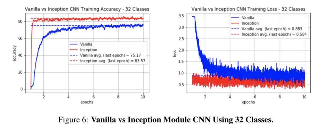
The first is a vanilla CNN with three convolutional and max pooling layers followed by three fully connected layers. The convolutional layers use 3x3 windows while the maxpooling layers use 2x2 windows. The second is a more complex architecture with a convolutional layer followed by an inception module followed by another convolutional layer and then two fully connected layers. 3x3 windows are again used for the convolutional layers, and the fully connected layers reduce the number of the units to the corresponding number of classes.
An inception module enables multiple convolutions of varying size to run in parallel, allowing for more features to be learned at different scales. This provides the model more flexibility to determine for itself what size convolutional windows are best for extracting features. The multiple feature maps are then concatenated and scaled to the correct size for the final convolutional layer. The inception module in our network uses 1x1, 3x1, 1x3, and 3x3 windows along with different padding techniques to test a variety of configurations. In addition, the inputs to each feature map are normalized using batch normalization in order to control the distribution of the inputs and reduce overfitting. Since this model is more powerful in its ability to extract relevant features, we expect it to perform better at classification than the vanilla CNN.
For the vanilla LSTM, input sequences are directly fed into 2 stacked LSTM layers with 128 and 512 units respectively. The first LSTM layer is set with true return sequence, which means each input sequence will have correcsponding LSTM outputs. The second LSTM layer's return sequence is set to false, subsequently only one set of LSTM outputs. The LSTM layers are followed by 2 dense layers with 128 units and units with same number as classes from input respectively.
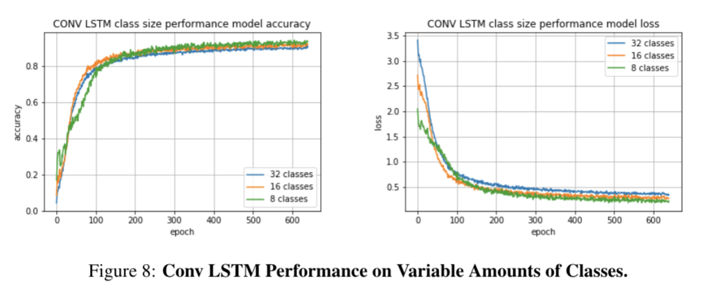
For the Convolution LSTM model, it has 3 extra Conv1D layers. The first two each has 48 and 64 channels of size 5x1 filters. The third Conv1D layer has 96 channels of 3x1 filters. The 2 LSTM and 2 dense layers have same structures as in vanilla LSTM.
The LSTM models were run in py3gym-gpu shell with tensorflow 1.4.0 and keras 2.1.5
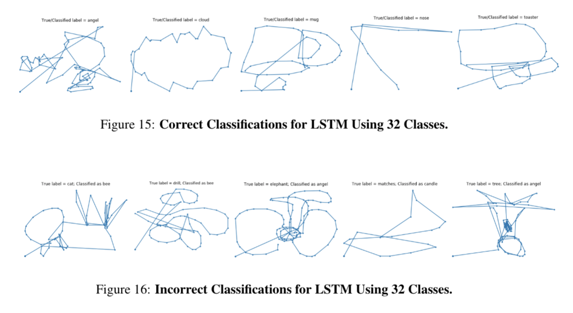
Below are the training/validation accuracy and loss curves throughout training ConvLSTM architecture and the final test accuracies for all of the CNN architectures. We also visualize the incorrect classifications for various models.


