55 Fundamental Unsupervised Learning Interview Questions

You can also find all 55 answers here 👉 Devinterview.io - Unsupervised Learning

1. What is unsupervised learning and how does it differ from supervised learning?

Unsupervised Learning involves modeling data with an unknown output and is distinguished from supervised learning by its lack of labeled training data.

Key Distinctions

Data Requirement

• Supervised: Requires labeled data for training, where inputs are mapped to specified outputs.
• Unsupervised: Lacks labeled data; the model identifies patterns, associations, or structures in the input data.

Tasks

• Supervised: Primarily used for predictions or for guiding inferences based on predefined associations.
• Unsupervised: Selects data associations or structures as primary objectives, often for exploratory data analysis.

Modeling Approach

• Supervised: Attempts to learn a mapping function that can predict the output, given the input.
• Unsupervised: Aims to describe the underlying structure or patterns of the input data, which can then be used for various analysis and decision-making tasks.

Common Techniques

• Supervised: Utilizes techniques like regression or classification.
• Unsupervised: Employs methods such as clustering and dimensionality reduction.

Data Labeling

• Supervised: Each data point is meticulously labeled with its corresponding output category.
• Unsupervised: Systems are left to identify structures or patterns on their own, without predefined labels.Formally, in an unsupervised task, we have a dataset $X$ from an unknown joint probability distribution $P(X,Y)$, and our objective is to understand the underlying structure of the data with only $X$ available. Conversely, in a supervised task, we have both $X$ and $Y$ available from the same probability distribution, and we want to train a model $f^*$ that minimizes the expected loss on unseen data, i.e., $\min_{f\in \mathcal{F}} \mathbb{E}_{(X,Y)}\left[ L(Y,f(X)) \right]$. Ultimately, the primary difference between the two is the nature of the available data and the corresponding learning objectives.

2. Name the main types of problems addressed by unsupervised learning.

Unsupervised Learning primarily focuses on solving three fundamental types of problems through pattern recognition, feature extraction, and grouping.

Fundamental Problem Types

Clustering

Definition: The task of dividing a dataset into groups, such that data points within the same group are more similar to each other compared to those in other groups.

Use-Cases: Segmentation of customers, document classification, image segmentation, and many more.

Association

Definition: The task of finding associations among items within a dataset. A classic example is market basket analysis, where the goal is to find items that are frequently purchased together.

Use-Cases: Recommendation systems, market basket analysis, and collaborative filtering.

Anomaly Detection

Definition: The identification of data instances that deviate from the norm. Also known as "outlier detection," this task is about identifying observations that differ significantly from the rest of the data.

Use-Cases: Fraud detection, network intrusion detection, and health monitoring.

3. Explain the concept of dimensionality reduction and why it's important.

Dimensionality reduction is a pivotal concept in the realms of data analysis, unsupervised learning, and machine learning in general. It refers to the process of reducing the number of random variables under consideration by obtaining a set of principal variables.

These principal variables capture the essential information of the original dataset, thus leading to a more streamlined and efficient approach to modeling and analysis.

Motivation for Dimensionality Reduction

1. Data Visualization: Reducing dimensions to 2D or 3D allows for visual representation.
2. Computational Efficiency: It's more efficient to compute operations in lower-dimensional spaces.
3. Noise and Overfitting Reduction: Reducing noise in the data can lead to more reliable models.
4. Feature Selection: It can help identify the most important features for prediction and classification tasks.

Techniques of Dimensionality Reduction

Two main methods achieve dimensionality reduction:

• Feature Selection: Directly choose a subset of the most relevant features.
• Feature Extraction: Generate new features that are combinations of the original features.

Feature Selection

Feature selection methods, including filter methods, wrapper methods, and embedded methods, aim to choose the most relevant features for the predictive model. For this purpose, various metrics and algorithms are employed, such as information gain, chi-square test, and Regularization.

Feature Extraction

• Principal Component Analysis (PCA): It generates new features as linear combinations of the old ones, with the goal of capturing the most variance in the data.

• Linear Discriminant Analysis (LDA): Particularly useful in supervised learning, it aims to maximize class separability.

• Kernel PCA: An extension of PCA, optimized for handling nonlinear relationships.

Unsupervised and Supervised Contexts

While feature extraction methods like PCA are often used in unsupervised learning because they're data-driven, feature selection methods can be effective in both supervised and unsupervised learning scenarios.

Code Example: PCA

Here is the Python code:

import numpy as np
from sklearn.decomposition import PCA

# Generate random data
np.random.seed(0)
X = np.random.normal(size=(20, 5))

# Perform PCA
pca = PCA(n_components=2)
X_reduced = pca.fit_transform(X)

# Show explained variance ratio
print(pca.explained_variance_ratio_)

4. What is clustering, and how can it be used to gain insights into data?

Clustering is an Unsupervised Learning technique used to identify natural groupings within datasets. It's valuable for data exploration, dimensionality reduction, and as a feature selection method.

Key Concepts

• Group Formation: Clustering algorithms assign data points into groups (clusters) based on their similarity, either globally or relative to a cluster center.

• Centrality: Most algorithms define clusters using a prototype, such as the mean or median of the data points. K-Means, for example, uses cluster centers.

• Distances: The concept of distance, often measured by Euclidean or Manhattan distance, is fundamental to grouping similar data points.

Data Exploration and Visualization

Clustering aids data exploration by illustrating natural groupings or associations within datasets. It is especially useful when the data's underlying structure is not clear through traditional means. Once the clusters are identified, visual tools like scatter plots can make the structures more apparent.

Dimensionality Reduction

Clustering can reduce high-dimensional data to an easily understandable lower dimension, often for visualization (e.g., through t-Distributed Stochastic Neighbor Embedding, t-SNE) or to speed up computations.

Feature Selection

By exploring clusters, you can determine the most discriminating features that define each cluster, aiding in feature selection and data understanding. For instance, these influential features can be used to build predictive models.

Use Case: Retail Analytics

Clustering can be instrumental in retail analytics for:

1. Behavior Segmentation: Based on purchasing or browsing behaviors, customers are grouped into segments. This can lead to insights such as the identification of "frequent buyers" or "window shoppers."

2. Inventory Management: Clustering customers based on purchase history or preferences helps in optimizing product offerings and stock management.

3. Marketing Strategies: Understand what products or offers attract different customer clusters, leading to better targeted marketing campaigns.

5. Can you discuss the differences between hard and soft clustering?

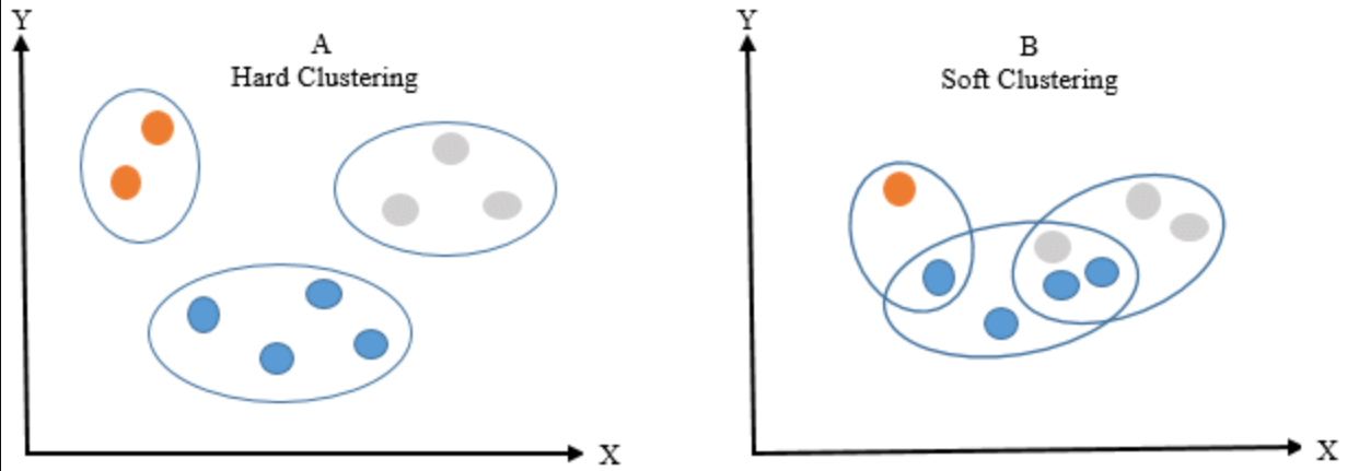
Hard clustering assigns each point to exactly one cluster. In contrast, soft clustering provides a probability or likelihood that a point belongs to one or more clusters. A popular technique for soft clustering is the Expectation-Maximization (EM) algorithm, often used in Gaussian Mixture Models (GMMs).

Common Techniques

• K-Means: Famous for hard clustering, it assigns each point to the nearest cluster center.
• Gaussian Mixture Models (GMMs): Associative with soft clustering, GMMs model clusters using multivariate Gaussian distributions and calculate probabilities of points belonging to each cluster.

Visual Representation of Soft and Hard Clustering

Mathematics Behind GMM

A Gaussian Mixture Model (GMM) models probability distributions of data points localized about their respective cluster means. The likelihood, often denoted as $P(z | \mathbf{x})$, gives the probability of a point $\mathbf{x}$ belonging to cluster $z$.

Mixture Model

Formally, the model is given as:

$$ P(\mathbf{x}) = \sum_{z=1}^{K} P(z) : P(\mathbf{x} | z) $$

Here, $P(z)$ represents the prior probability of a point belonging to a cluster $z$, while $P(\mathbf{x} | z)$ denotes the likelihood of observing $\mathbf{x}$ given it belongs to cluster $z$.

In the context of GMMs, the likelihood is described using multivariate Gaussian distributions:

$$ P(\mathbf{x} | z) = \mathcal{N}(\boldsymbol{\mu}_z, \Sigma_z) $$

Where $\boldsymbol{\mu}_z$ is the mean vector and $\Sigma_z$ is the covariance matrix of the Gaussian component corresponding to cluster $z$.

GMM Estimation

The Expectation-Maximization (EM) algorithm iteratively carries out two steps:

• Expectation (E-Step): For each data point, it calculates the probability of it belonging to each cluster. This step involves finding the responsibilities $\gamma(z)$ of each cluster for each point.
• Maximization (M-Step): Updates the parameters, such as cluster means and covariances, using the computed responsibilities.

Code Example: Hard vs Soft Clustering

Here is the Python code:

from sklearn.cluster import KMeans, AgglomerativeClustering
from sklearn.mixture import GaussianMixture

# Hard Clustering with K-Means

kmeans = KMeans(n_clusters=3)
kmeans.fit(data)
kmeans_labels = kmeans.labels_

# Soft Clustering with GMM

gmm = GaussianMixture(n_components=3)
gmm.fit(data)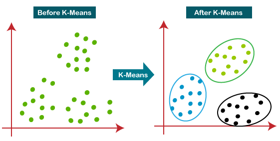
gmm_probs = gmm.predict_proba(data)

6. Describe the K-means clustering algorithm and how it operates.

K-means clustering is a widely-used unsupervised learning algorithm for partitioning $n$-dimensional data points into $k$ clusters.

Algorithm Steps

1. Initialize Centroids: Assign $k$ data points randomly as the initial centroids.

2. Distance Calculation: For each data point, calculate its distance to all centroids.

3. Cluster Assignment: Assign each data point to the nearest centroid's cluster.

4. Centroid Recalculation: Update the position of each centroid as the mean of the data points in its cluster.

5. Convergence Check: Repeat steps 2-4 as long as the centroids keep changing. Convergence typically occurs when the sum of Euclidean distances between previous and new centroids become close to 0.

Pseudocode

Choose k initial centroids
while centroids are changing:
    Assign each data point to the nearest centroid
    Calculate new centroids as the mean of data points in each cluster

Visual Representation

Code Example: K-means on 2D Data

Here is the Python code:

import numpy as np
from sklearn.cluster import KMeans
import matplotlib.pyplot as plt

# Simulated 2D data points
X = np.array([[1, 2], [1, 4], [1, 0],
              [4, 2], [4, 4], [4, 0]])

# Initializing KMeans
kmeans = KMeans(n_clusters=2, random_state=0)

# Fitting the model
kmeans.fit(X)

# Visualizing the clusters
plt.scatter(X[:,0], X[:,1], c=kmeans.labels_, cmap='viridis')
plt.scatter(kmeans.cluster_centers_[:,0], kmeans.cluster_centers_[:,1], c='red', marker='x')
plt.show()

7. What is the role of the silhouette coefficient in clustering analysis?

The silhouette coefficient serves as an indicator of cluster quality and provides a way to quantify separation and homogeneity within clusters.

It's particularly useful in scenarios where the true label of the data is unknown, which is often the case with unsupervised learning. A higher silhouette coefficient signifies better-defined clusters.

Calculating the Silhouette Coefficient

The silhouette coefficient is a metric $s$ for each sample, defined as the difference between the mean intra-cluster distance $a$ and the nearest-cluster distance $b$ divided by the maximum of the two:

$$ s = \frac{b - a}{\max (a, b)} $$

The coefficient ranges from -1 to 1, where:

• 1 indicates that the sample is well-matched to its own cluster and poorly matched to neighboring clusters.
• -1 indicates that the sample is poorly matched to its assigned cluster and may be more suited to a neighboring cluster.

Benefits of the Silhouette Coefficient

• Easily Computable: Identifying optimal primary and secondary clusters by maximizing silhouette score is computationally less demanding than cross-validating.
• Visual Assessment: Silhouette plots help visualize the silhouette scores for individual data points.
• Cluster Shape Consideration: The silhouette coefficient considers both cluster cohesion and separation, making it suitable for clusters of varied shapes and sizes.

Code Example: Silhouette Coefficient

Here is the Python code:

from sklearn.datasets import make_moons
from sklearn.cluster import KMeans
from sklearn.metrics import silhouette_samples, silhouette_score
import matplotlib.pyplot as plt
import numpy as np

# Generating synthetic data
X, _ = make_moons(n_samples=500, noise=0.1)

# Range of cluster numbers to test
range_n_clusters = [2, 3, 4, 5, 6]

for n_clusters in range_n_clusters:
    # Initialize KMeans with n_clusters
    clusterer = KMeans(n_clusters=n_clusters, random_state=10)
    cluster_labels = clusterer.fit_predict(X)
    
    # Obtain silhouette score for this KMeans model
    silhouette_avg = silhouette_score(X, cluster_labels)
    print(f"For n_clusters = {n_clusters}, the average silhouette score is: {silhouette_avg}")

    # Obtain silhouette values for each data point
    sample_silhouette_values = silhouette_samples(X, cluster_labels)

    y_lower = 10
    for i in range(n_clusters):
        # Aggregate the silhouette scores for samples belonging to
        # cluster i, and sort them
        ith_cluster_silhouette_values = \
            sample_silhouette_values[cluster_labels == i]

        ith_cluster_silhouette_values.sort()

        size_cluster_i = ith_cluster_silhouette_values.shape[0]
        y_upper = y_lower + size_cluster_i

        color = cm.nipy_spectral(float(i) / n_clusters)
        ax1.fill_betweenx(np.arange(y_lower, y_upper),
                          0, ith_cluster_silhouette_values,
                          facecolor=color, edgecolor=color, alpha=0.7)

        # Label the silhouette plots with their cluster numbers at the middle
        ax1.text(-0.05, y_lower + 0.5 * size_cluster_i, str(i))

        # Compute the new y_lower for next plot
        y_lower = y_upper + 10  # 10 for the 0 samples

    ax1.set_title("The silhouette plot for the various clusters.")
    ax1.set_xlabel("The silhouette coefficient values")
    ax1.set_ylabel("Cluster label")

    # The vertical line for average silhouette score of all clusters
    ax1.axvline(x=silhouette_avg, color="red", linestyle="--")

    ax1.set_yticks([])  # Clear the yaxis labels / ticks
    ax1.set_xticks([-0.1, 0, 0.2, 0.4, 0.6, 0.8, 1])

    plt.show()

8. Explain the DBSCAN algorithm. What advantages does it offer over K-means?

Density-Based Spatial Clustering of Applications with Noise (DBSCAN) and K-means are popular clustering algorithms. While K-means is sensitive to outliers and requires the number of clusters $k$ to be predefined, DBSCAN can handle such challenges more effectively.

Key Elements of DBSCAN

1. Core Points: Data points with at least a minimum number of points $\text{MinPts}$ within a specified distance $\varepsilon$ are considered core points.

2. Border Points: Data points that are within $\varepsilon$ distance of a core point but do not themselves have the minimum number of points within $\varepsilon$ are considered border points.

3. Noise Points: Data points that are not core points or border points are considered noise points, often denoted as outliers.

DBSCAN Process in Clustering

1. Point Classification: Each point in the dataset is classified as either a core point, border point, or noise point.

2. Point Connectivity: Core points are directly or indirectly connected through other core points. This connectivity helps in the formation of clusters.

3. Cluster Formation: Clusters are formed by aggregating core points and their directly reachable non-core points (which are border points).

Advantages Over K-means

• Flexibility: DBSCAN does not make assumptions about the shape of the clusters, allowing it to find clusters of various shapes. In contrast, K-means assumes spherical clusters.

• Automatic Outlier Detection: K-means does not inherently identify outliers, while DBSCAN naturally captures them as noise points.

• No Need for Predefined Cluster Count: K-means often requires the user to specify the number of clusters, which is not the case with DBSCAN.

• Ability to Handle Uneven Cluster Densities: DBSCAN can be more robust when clusters have different densities, whereas K-means assumes all clusters have similar variance.

• Reduced Sensitivity to the Initialization: K-means results can vary based on different initializations, whereas DBSCAN's performance is less influenced by initial conditions.

• Robustness to Noise: DBSCAN is less influenced by noisy data points, ensuring they end up as noise.

Key Parameters in DBSCAN

• Epsilon $(\varepsilon)$: This distance parameter defines the neighborhood around a point. Points within this distance from another point are considered as part of the same cluster.
• MinPts: The minimum number of points within the neighborhood $\varepsilon$ for a point to be classified as a core point.

Performance Considerations

• Time Complexity: DBSCAN's time complexity is often linear with the number of samples, making it efficient for large datasets.

• Scalability: The algorithm can become less efficient with growing numbers of dimensions and clusters.

Code Example: DBSCAN using scikit-learn

Here is the Python code:

from sklearn.cluster import DBSCAN
from sklearn.datasets import make_blobs
import matplotlib.pyplot as plt

# Generate sample data
X, _ = make_blobs(n_samples=250, centers=5, cluster_std=1.0, random_state=42)

# Initialize and fit DBSCAN
dbscan = DBSCAN(eps=1, min_samples=5)
dbscan.fit(X)

# Visualize the clusters
plt.scatter(X[:, 0], X[:, 1], c=dbscan.labels_, cmap='viridis', s=50, alpha=0.7)
plt.title('DBSCAN Clustering')
plt.show()

9. How does the hierarchical clustering algorithm work, and when would you use it?

Hierarchical Clustering is an unsupervised learning algorithm that forms clusters by either combining data points into progressively larger clusters (agglomerative approach) or by breaking clusters into smaller ones (divisive approach). This process is visualized using a dendrogram.

Key Algorithmic Steps

1. Data Point Initialization: Each data point is considered a separate cluster.
2. Distance Matrix Calculation: A matrix capturing the distance between each pair of clusters is established. Various distance metrics can be applied. For numerical data, the Euclidean distance is often used, while for other data types, specialized methods may be necessary.
3. Cluster Merger (Agglomerative) / Split Criteria (Divisive): This involves determining which clusters to merge or split, based on proximity.
4. Repeat Steps 2-3: The process iterates until the stopping condition is met.
5. Dendrogram Generation: This detailed tree-like structure shows the clustering process.

Both Agglomerative and Divisive Methods

• Agglomerative: This starts with each data point as a single-point cluster and merges the closest clusters until all points are part of one cluster. The linkage, or method used to merge clusters, influences the algorithm.

  • Single Linkage: Based on the smallest distance between clusters.
  • Complete Linkage: Based on the maximum distance between clusters.
  • Average Linkage: Based on the average distance between clusters.

• Divisive: This is the opposite of agglomerative, starting with all data points in a single cluster and iteratively breaking them down.

Dendrogram-Based Cluster Selection

The dendrogram is a powerful tool that shows the order and distances at which clusters are merged. It's a valuable visual aid for choosing the number of clusters, especially in scenarios where direct measurements, such as the silhouette score, aren't applicable.

To identify the optimal number of clusters:

1. Set a Threshold: Use the dendrogram to identify the level at which the cluster count is most meaningful.

2. Cut the Dendrogram: Trim the tree at the chosen level to produce the required number of clusters.

3. Visualize and Validate: Examine the resulting clusters to determine if they are well-separated and if the chosen cluster count makes sense in the given context.

Code Example: Dendrogram and Cluster Selection

Here is the Python code:

import numpy as np
from scipy.cluster import hierarchy
import matplotlib.pyplot as plt

# Generate random data for demonstration
np.random.seed(123)
data = np.random.rand(10, 2)

# Perform hierarchical clustering
linkage_matrix = hierarchy.linkage(data, method='average')
dendrogram = hierarchy.dendrogram(linkage_matrix)

# Visualize dendrogram
plt.title('Dendrogram')
plt.xlabel('Data Points')
plt.ylabel('Distance')
plt.show()

10. What is the difference between Agglomerative and Divisive hierarchical clustering?

Let's explain the differences between Agglomerative and Divisive hierarchical clustering methods, and then describe their performance levels.

Algorithmic Approaches

• Agglomerative Clustering: Starts with each data point as a cluster and merges them based on similarity metrics, forming a tree-like structure.
• Divisive Clustering: Begins with all data points in a single cluster and then divides the clusters into smaller ones based on dissimilarity metrics.

Performance Considerations

• Computational Efficiency: Divisive clustering generally requires more computational resources than agglomerative clustering due to the top-down nature of the division algorithm.

• Memory Utilization: Agglomerative clustering can be more memory-efficient since it builds the hierarchy from a bottom-up approach, while divisive clustering builds from the top-down, potentially needing more memory to store interim results.

• Time Complexity: Both techniques are computationally demanding. Agglomerative clustering has a time complexity generally of $O(n^3)$, while divisive clustering can be even more computationally expensive.

• Quality of Clusters: Agglomerative method can create uneven cluster sizes since the dendrogram "tree" can have imbalanced splits. Divisive clustering tends to create clusters of more even sizes.

Use Cases

• Agglomerative Clustering: Often used when the number of clusters is not known in advance. It’s a go-to method for tasks such as customer segmentation, document clustering, and genetic research.
• Divisive Clustering: Less commonly used than agglomerative methods. It can be suitable in scenarios where there is a priori knowledge about the number of clusters, but this information is not employed in the clustering process.

11. Explain the working of Principal Component Analysis (PCA).

Principal Component Analysis (PCA) is a fundamental dimensionality reduction technique used in unsupervised learning to identify the most critical sources of variance in the data.

Key Concepts

Variance-Covariance Matrix

The Variance-Covariance Matrix $\Sigma$ defines the relationships between all pairs of features. Its values show how features vary with and influence one another.

Eigenvalues and Eigenvectors

PCA computes the eigenvectors of $\Sigma$, which correspond to the principal components of the data, and their associated eigenvalues, quantifying the variance along each eigenvector.

Feature Transformation

The computed eigenvectors form a feature transformation matrix $W$, allowing for the projection of the original data into a more informative eigenbasis.

Cumulative Explained Variance

Eigenvalues capture the relative importance of each principal component, providing a means to select a subset that retains a desired percentage of the dataset's total variance.

Algorithm Steps

1. Data Standardization: It's essential to scale the data before performing PCA to ensure that features on different scales contribute equally to the analysis.

2. Covariance Matrix Calculation: The covariance matrix $\Sigma$ is constructed by evaluating the pair-wise feature covariances.

3. Eigenvalue Decomposition: PCA seeks the eigenvectors and eigenvalues of the covariance matrix. Both are calculated in one step, thus speeding up the process.

4. Eigenvector Sorting: The eigenvectors, representing the principal components, are ordered based on their associated eigenvalues, from highest to lowest.

Variance Retention and Elbow Method

The cumulative explained variance is a fundamental concept in understanding model fitness and feature uniqueness. After ranking eigenvalues, the cumulative explained variance at each eigenvalue provides insight into the proportion of variance retained by considering a given number of principal components.

The elbow method visualizes the eigenvalue magnitudes and allows you to determine the "elbow point," indicating when each subsequent principal component contributes less significantly to the overall variance. Choosing principal components before this point can help balance information retention with dimensionality reduction.

Code Example: Scikit-Learn

Here is the Python code:

from sklearn.decomposition import PCA

# Assuming X is your data
# Instantiate the PCA object
pca = PCA()

# Fit and transform your data to get the principal components
X_pca = pca.fit_transform(X)

# Get the eigenvalues and the percentage of variance they explain
eigvals = pca.explained_variance_
explained_var = pca.explained_variance_ratio_

12. Describe t-Distributed Stochastic Neighbor Embedding (t-SNE) and its use cases.

t-distributed Stochastic Neighbor Embedding (t-SNE) is a popular technique for visualizing high-dimensional data in lower dimensions such as 2D or 3D, by focusing on the relationships between neighborhood points. In particular, it preserves local data structures.

Key Components

• Kullback-Leibler (KL) Divergence: Measures how a distribution $P$ differs from a target distribution $Q$. t-SNE aims to minimize the difference between the distributions of pairwise similarities in input and output spaces.

• Cauchy Distribution: A key component of the algorithm. It dictates the probability that two data points will be deemed neighbors.

Algorithm Steps

1. Create Probabilities: Compute pairwise similarities between all data points in the high-dimensional space using a Gaussian kernel.

$$ p_{j\mid i} = \frac{\exp\left(-\frac{{\lVert x_i - x_j \rVert}^2}{2\sigma_i^2}\right)}{\sum_{k\neq i}\exp\left(-\frac{{\lVert x_i - x_k \rVert}^2}{2\sigma_i^2}\right)} $$

2. Initialize Low-Dimensional Embedding: Sample each point from a normal distribution.

3. Compute T-Distributions: Calculate pairwise similarities in the low-dimensional space, again using a Gaussian kernel.

$$ q_{j\mid i} = \frac{1}{{1 + \lVert y_i - y_j \rVert^2}} $$

4. Optimize: Employ gradient descent on the cost function to align the low-dimensional embeddings to the high-dimensional pairwise similarities.

Use Cases

• Image Analysis: It can identify semantic features in images.
• Text Mining: Useful for exploring word contexts and relationships for context-rich text analysis.
• Biology and Bioinformatics: For analyzing gene expression or drug response datasets to uncover underlying structures.
• Astronomy: To study patterns in celestial data.

Limitations

• Non-deterministic Nature: t-SNE can generate different visualizations for the same dataset.
• Sensitivity to Parameters: It requires careful tuning.
• Computational Demands: The algorithm can be slow when dealing with large datasets, often requiring a parallelized implementation or sampling from the dataset.

13. How does Linear Discriminant Analysis (LDA) differ from PCA, and when would you use each?

While Linear Discriminant Analysis (LDA) and Principal Component Analysis (PCA) both operate in the domain of unsupervised learning for feature reduction, they each have distinctive approaches and are suited to different tasks.

Core Distinctions

Methodology

• LDA: It maximizes the inter-class variance and minimizes the intra-class variance.
• PCA: It selects the dimensions with maximum variance, regardless of class separation.

Supervision

• LDA: Supervised learning method that requires class labels.
• PCA: Unsupervised technique that operates independently of class labels.

Objective

• LDA: Emphasis on optimizing for class separability.
• PCA: Focuses on variance across the entire dataset.

Feature Selection

• LDA: Aims to identify the features that discriminate well between classes.
• PCA: Retains features that explain dataset variance.

Practical Use-Cases

• LDA: Often used in the context of multi-class classification problems to improve inter-class separability.
• PCA: Widely employed in numerous applications, including for data visualization and feature reduction in high-dimensional datasets.

14. What is the curse of dimensionality and how does it affect machine learning models?

The Curse of Dimensionality describes the practical and theoretical challenges that arise when dealing with high-dimensional data, especially in the context of Black Box Optimization (BBO) and machine learning. As the number of dimensions or features in a dataset increases, the volume of the space data resides in grows exponentially, often causing more harm than allowing for clearer separations.

Key Challenges

1. Data Sparsity: The actual data filled in the high-dimensional space becomes sparse. Most data separation and machine learning models require a certain amount of data to function effectively.
2. Distance Computations: The computation of distances becomes less meaningful as the number of features increases. Traditional Euclidean distances, for example, become less discriminating.
3. Parameter Estimation: As the number of dimensions to estimate parameters and reduce risk or error increases, models require more data or experience a decrease in precision.
4. Model Complexity: With the increase in dimensions, the model's complexity also grows. This often leads to overfitting.

Implications for Machine Learning

1. Reduced Generalization: With a plethora of features, it becomes easier for a model to "memorize" the data, resulting in poor generalization to new, unseen data.

2. Increased Computational Demands: The computational requirements of many machine learning models, such as K-means, increase with the number of dimensions. This can make model training much slower.

3. Feature Selection and Dimensionality Reduction: In response to the curse of dimensionality, feature selection or techniques like Principal Component Analysis (PCA) can help reduce the number of dimensions, making the data more manageable for models.

4. Data Collection: The curse of dimensionality emphasizes the importance of thoughtful data collection. Having more features doesn't always equate to better models.

5. Data Visualization: Humans have a hard time visualizing data beyond three dimensions. While not a direct challenge for the model, it becomes a challenge for the model's users and interpreters.

Techniques to Mitigate the Curse of Dimensionality

1. Feature Selection: Here, one can manually or algorithmically select a subset of features that are most relevant to the problem at hand.
2. Regularization: Techniques like Lasso or Ridge regression reduce the impact of less important features.
3. Feature Engineering: Creating new, useful features from existing ones.
4. Model Selection and Evaluation: Choosing models that are robust in high-dimensional settings and that can be effectively evaluated with limited data.

Code Example: SelectKBest in Scikit-Learn

Here is the Python code:

from sklearn.datasets import load_iris
from sklearn.feature_selection import SelectKBest, chi2

# Load the iris dataset
iris = load_iris()
X, y = iris.data, iris.target

# Reduce the number of features to 2 using SelectKBest
X_new = SelectKBest(chi2, k=2).fit_transform(X, y)

15. Explain what an autoencoder is and how it can be used for dimensionality reduction.

An autoencoder is an unsupervised learning architecture that learns to encode and then decode input data, aiming to reconstruct the input at the output layer.

This architecture consists of an encoder, which maps the input to a hidden layer, and a decoder, which reconstructs the input from the hidden layer. The autoencoder is trained to minimize the reconstruction error between the input and the output.

Workflow of an Autoencoder

1. Encoding:

   • The input data is compressed into a lower-dimensional latent space using the encoder.
   • The output of the encoder typically represents the data in a reduced and more salient feature space.

2. Decoding:

   • The latent representation is then reconstructed back into the original data space using the decoder.

Types of Autoencoders

1. Vanilla Autoencoder:

   • The simplest form of an autoencoder with a single hidden layer.

2. Multilayer Autoencoder:

   • Features multiple hidden layers, often following an hourglass structure where the number of nodes reduces and then increases.

3. Convolutional Autoencoder:

   • Utilizes convolutional layers in both the encoder and decoder, designed for image data with spatial hierarchies.

4. Variational Autoencoder (VAE):

   • Introduces a probabilistic framework, which assists in continuous, smooth latent space interpolation.

5. Denoising Autoencoder:

   • Trains the autoencoder to denoise corrupted input, which often results in more robust feature extraction.

6. Sparse Autoencoder:

   • Encourages a sparsity constraint in the latent representation, promoting disentangled and useful features.

7. Adversarial Autoencoder:

   • Incorporates a generative adversarial network (GAN) architecture to improve the quality of latent space representation.

8. Stacked Autoencoder:

   • Consists of multiple autoencoders stacked on top of each other, with the output of each serving as input to the next, often leading to improved reconstruction and feature learning.

Dimensionality Reduction with Autoencoders

Autoencoders are trained without explicit supervision, learning to capture the most salient features of the input data while ignoring noise and other less relevant information. As a result, they can effectively reduce the dimensionality of the input data.

After training, by using just the encoder part of the autoencoder, you can obtain the reduced-dimensional representations of the input data. Because this encoding step serves as a dimensionality reduction operation, autoencoders are considered a type of unsupervised dimensionality reduction technique.

Intuitions

The effectiveness of autoencoders for dimensionality reduction stems from their ability to:

• Elicit non-linear relationships through the use of non-linear activation functions.
• Discover intricate data structures like manifolds and clusters.
• Automatically select and highlight the most pertinent attributes or components of the data.

Code Example: Building an Autoencoder

Use Keras to create a simple autoencoder for MNIST data:

Here is the Python code:

from tensorflow.keras.layers import Input, Dense
from tensorflow.keras.models import Model

# Define the architecture
input_layer = Input(shape=(784,))
encoded = Dense(32, activation='relu')(input_layer)
decoded = Dense(784, activation='sigmoid')(encoded)

# Construct and compile the model
autoencoder = Model(input_layer, decoded)
autoencoder.compile(optimizer='adam', loss='binary_crossentropy')

# Train the model
autoencoder.fit(X_train, X_train, epochs=5, batch_size=256, shuffle=True)

# Extract the encoder for dimensionality reduction
encoder = Model(input_layer, encoded)
encoded_data = encoder.predict(X_test)

Explore all 55 answers here 👉 Devinterview.io - Unsupervised Learning