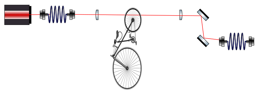
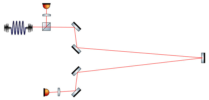
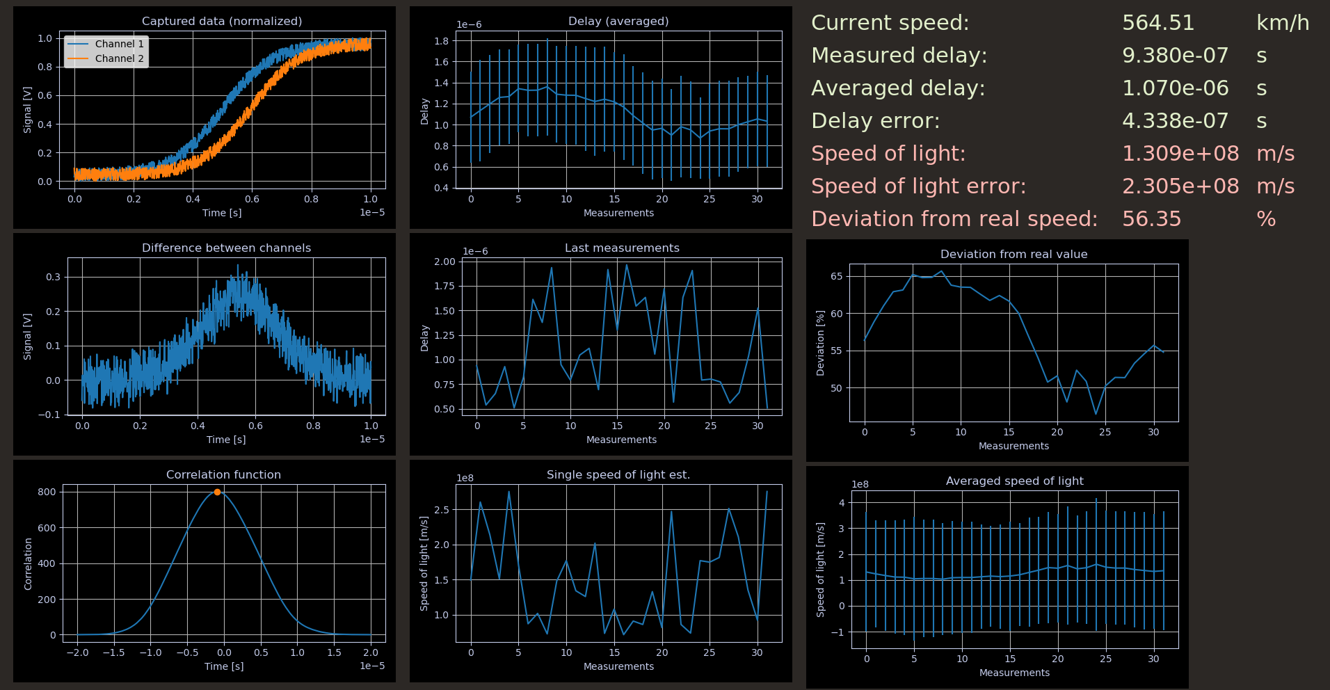
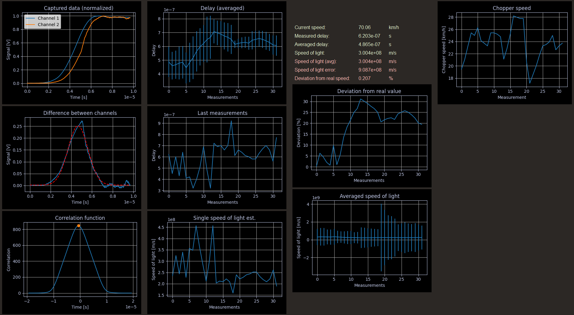
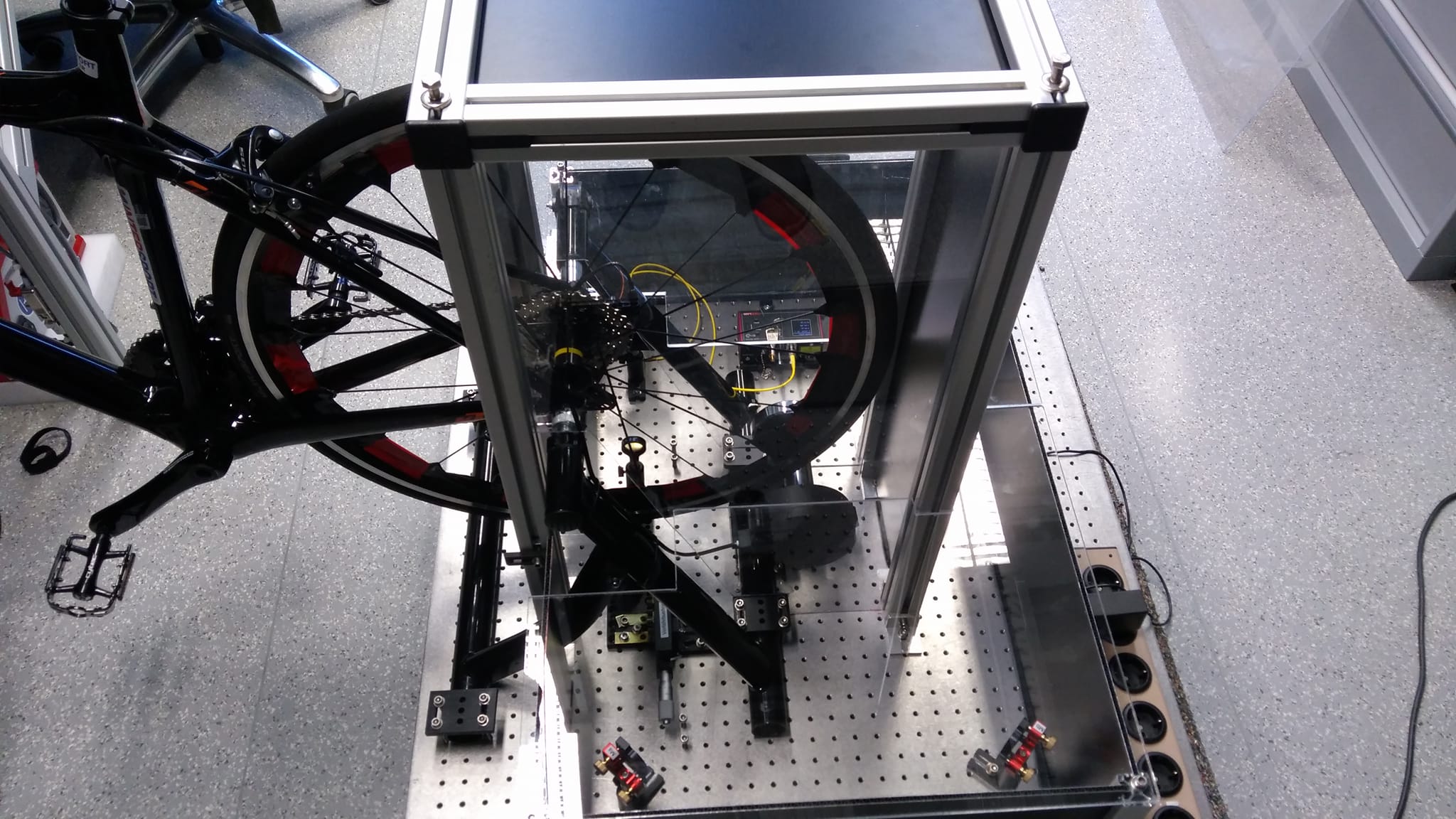
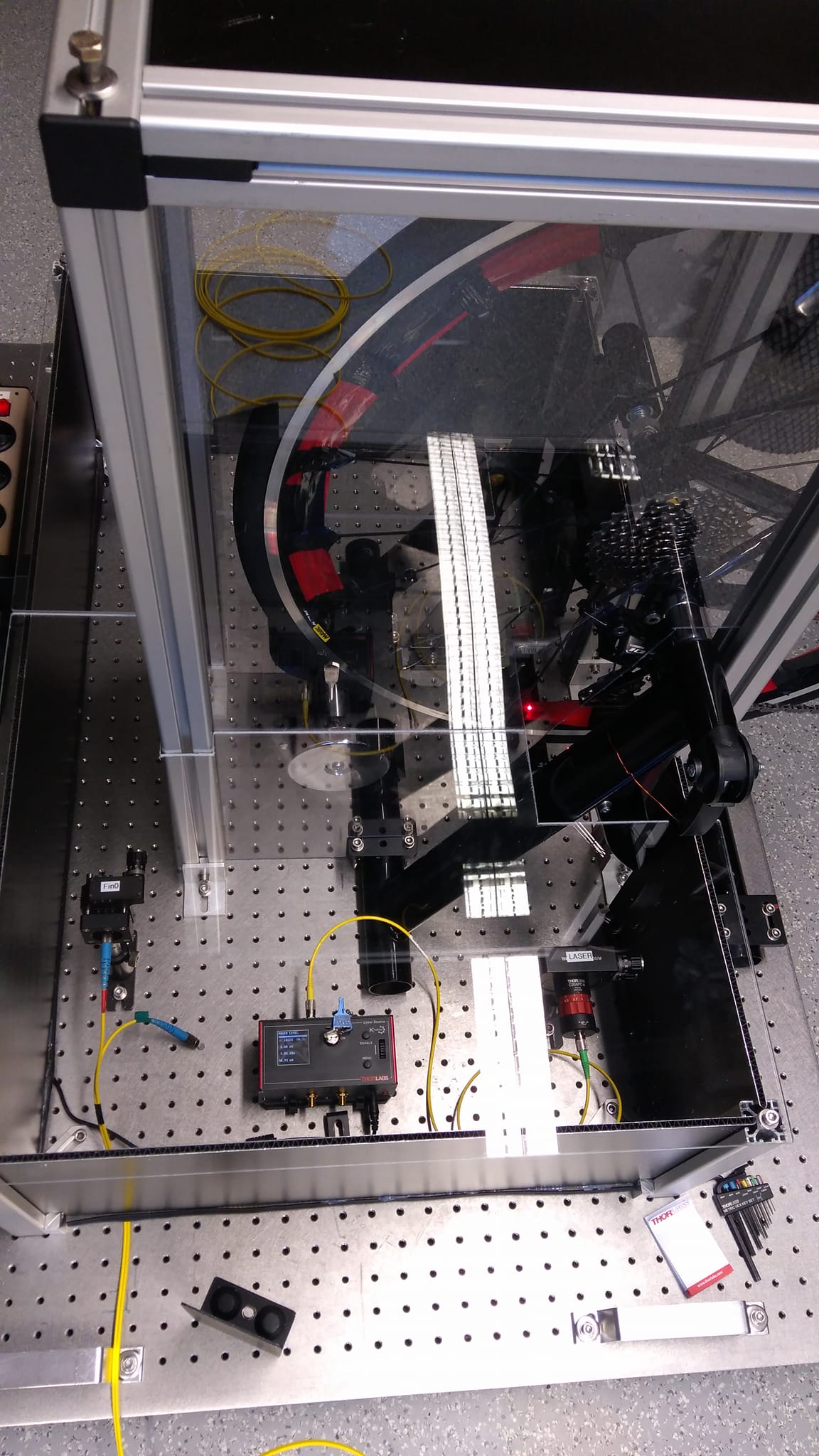
This is the frontend to the speed of light outreach project. This project has been developed to measure the speed of light similar to the idea that Hippolyte Fizeau developed in 1848. In contrast to his experiment in this case a little cheat is used - a bicycle works as chopper to produce a sharp difference in light intensity of a laser source. The light travels through two arms of the experiment - one being only a few meters away from the chopper, the other being about hundred meters away. The signal of both pulses is recorded on photodiodes and sampled by a fast oscilloscope (this is where the cheating comes in - we have a definition of time and fast direct sampling).
Since this project has been developed to increase the interest in science and let people participate actively during exhibitions it's by no way a precision measurement - it's more of a (working) experiment that people can look at, play with and grasp the idea of light traveling at finite speeds.
This application:
- Gathers data from the oscilloscope
- Visualizes the samples
- Calculates a cross correlation of the symmetrized periodicalized recorded function
- Estimates the speed of light from this correlation function by doing a simple peak search
- Does averaging over the estimated speed of light and visualized this.
The experimental setup consists of two basic parts:
- A chopper assembly - where a bicycle is used (or any other kind of chopper)
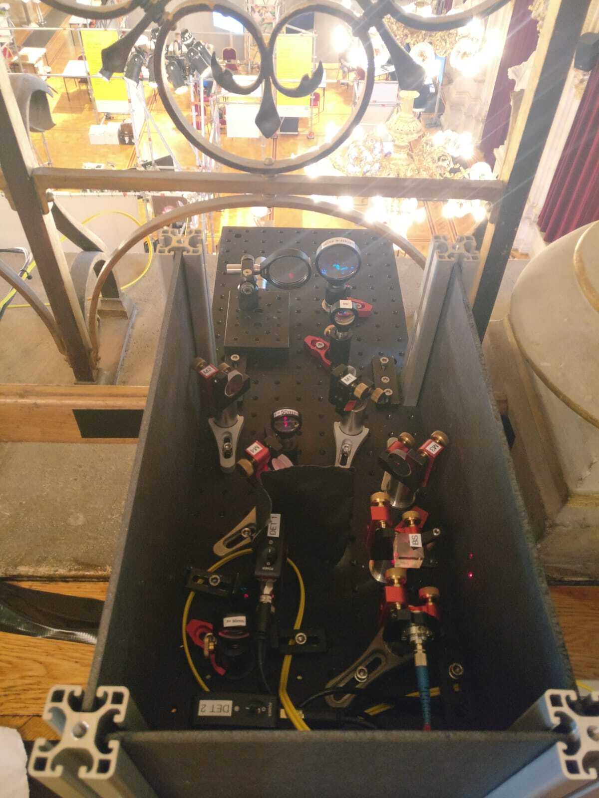
- A beam splitter and photodiode assembly as well as a long beam line
Installation can be done via the PyPi package:
pip install outreachspeedoflight-tspspi
This also installs the outreachspeedoflightgui script / executable that
can then directly be executed using
outreachspeedoflightgui
To upgrade an older installation one can also directly use pip:
pip install --upgrade outreachspeedoflight-tspspi
The data acquisition module configures the communication with the MSO5000 oscilloscope.
Example configuration:
{
	"osci" : {
		"ip" : "10.0.0.196",
		"port" : 5555,
		"sperdiv" : 1e-6,
		"trigch" : 1,
		"triglvl" : 0.5,
		"ch1" : {
			"offset" : -1.48,
			"scale" : 0.5
		},
		"ch2" : {
			"offset" : -0.920,
			"scale" : 0.5
		},
		"maxqueryrate" : 0.5
	},
	"chopper" : {
		"diameter" : 68e-2
	},
	"path" : {
		"length" : 144,
		"n" : 1.0
	},
	"loglevel" : "debug",
	"mode" : "continuous"
}
The osci section configured the MSO5000 oscilloscope:
- Connectivity:
- The
ipfield can be either the IP or hostname as string portis optional and defaults to5555
- The
- Optional Horizontal axis (time) configuration:
sperdivspecifies the seconds per division on the horizontal axis. This has to be a value supported by the oscilloscope
- Optional Trigger configuration:
trigchselects a channel (1 or 2) for the trigger to act ontriglvlselects the trigger level in volts.
- Optional channel configuration
ch1andch2:- One can specify an
offsetin volts - and a
scalespecified in volts per division that has to be a supported value by the oscilloscope
- One can specify an
- A optional maximum query rate in Hz (i.e. queries per second) that can be used to limit the amount of queries to the oscilloscope since at some point it won't update it's own local display anymore due to prioritization of network queries. When not specified the application queries as fast as possible.
The chopper section configures the chopper that is used. For our
experimental setup this can be a bicycle or a simple wooden wheel:
diameterconfigures the diameter of the wheel in meters. This is only used for velocity calculation from trigger rate assuming that only one trigger is issued per cycle.
An important configuration is the path. This describes the free path
the light pulse is traveling through. One can describe the length in
meters and the refractive index n (1 for air or vacuum or about 1.4 for
glass fibers)
At last one can select between two modes of operation using the mode
parameter:
triggereduses the scope in single trigger mode and re-arms when ready to gather more data. This ensures that both channels correspond to the same event but looks less real time on the oscilloscopes local display.continuouscontinuously samples on the scope and queries data as fast as possible.
Example configuration:
{
	"lang" : "de",
	"loglevel" : "debug",
	"lastsamples" : 24,
	"averagecount" : 4,
	"plotsize" : {
		"x" : 550,
		"y" : 430
	},
	"mainwindowsize" : {
		"x" : 2560,
		"y" : 1500
	},
	"difffit" : {
		"enable" : "true",
		"primary" : "false",
		"dump" : "true"
	},
	"movingaverage" : 48,
	"textfontsize" : 23
}
The user interface can be configured using gui.conf. This allows one to configure
some analysis parameters:
- The number of last measurements to be shown using
lastsamples - The number of measurements to include in rolling average
averagecount - A optional fit of a Gaussian function into the difference signal (that can
also be used instead of the autocorrelation function to detect the time delay).
This is done in the
difffitdictionary:enableis set to the strings"true"or"false". When set to true fitting is enabled. Keep in mind this is numerically more demanding than the other methodsprimarycan be either"true"or"false". If set to true the FWHM of the fit is used as measure for time delay of the signals and thus to calculate the speed of light. When set to"false"the fit is only plotted and the speed is still calculated using the cross correlation of both signalsdumpis set to"true"to dump fitting result and parameters to the standard output (for debugging purposes)
- To handle noisy signals on the photodiodes
movingaveragecan be set to any integer value larger than 0 (or to 0 to disable the feature). It applies a moving average filter of the specified number of samples - and thus applies a low pass filter to the signal. textfontsizeallows one to tune the size of text fields on the user interface to match the display size
In addition one can directly configure some layout parameters:
plotsizewithxandyparameters directly scales all plotsmainwindowsizewithxandyparameters scales the main window as initially created.
Note that invalid setting of those parameters might clip some graphs or cause some strange behavior of the user interface.
The highscore window can be configured using the highscore.conf configuration file.
Example configuration:
{
	"loglevel" : "debug",
	"highscorefile" : "/tmp/highscore.dat",
	"mainwindowsize" : {
		"x" : 1920,
		"y" : 1500
	},
	"tablesize" : {
		"x" : 1350,
		"y" : 250
	},
	"lang" : "de"
}
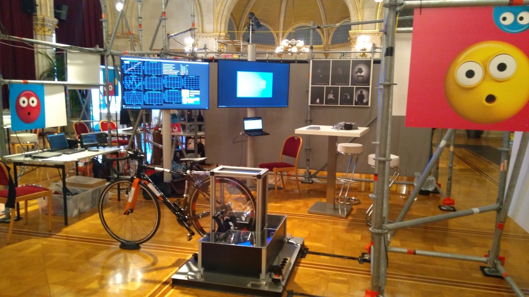
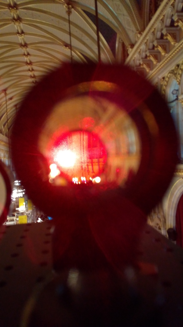
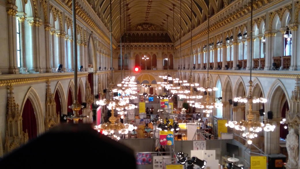
The Wiener Forschungfest 2022 that had been organized by the Wirtschaftsagentur Wien has been the first time our setup has been displayed. The event took place in Wiener Rathaus from 9. to 11. September 2022 and targeted mainly children at an age of 8 years or older and should focus on participation (thus the idea to use a bike as chopper) as well as showing possible carreer options in various areas of science. The beamline was 144m long (72 meters from one side of the city hall to the other) and passed over the heads of the people. Alignment and stability has been a little bit of a challenge due to instabilities of wooden floor but the setup turned out to be pretty accurate (at sub percent levels).
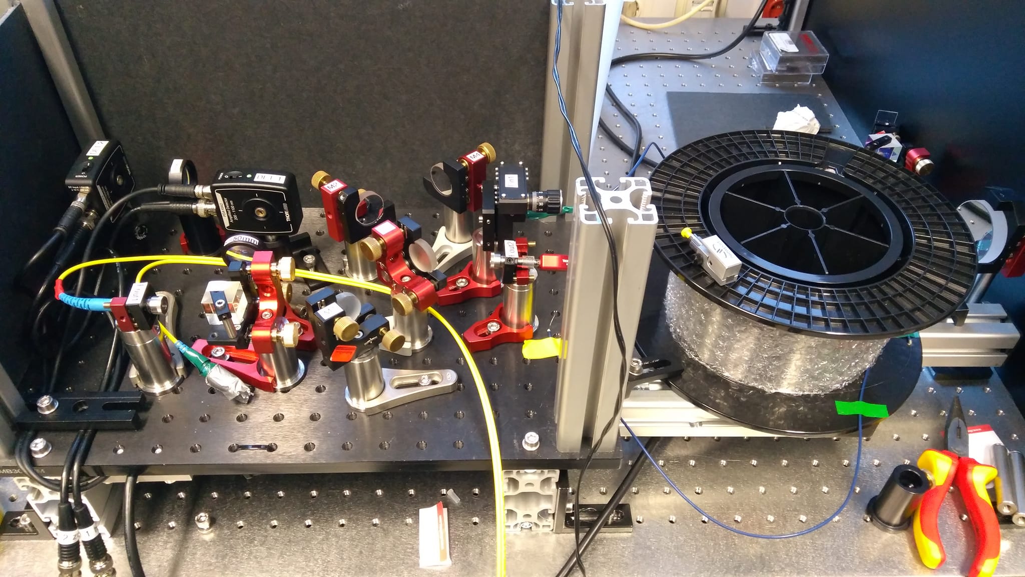
The telescope setup had been pretty simple - fiber coupler, non polarizing 50:50 beamsplitter cube, some mirrors to allow beam walking and alignment, one telescope lens assembly and one focus lens.
