-
Notifications
You must be signed in to change notification settings - Fork 30
benchmarking
R users have a few choices of how to connect to their MS Sql Server Database. The most commonly seen include:
-
RODBCused essentially Windows environment -
RJDBCto access from Linux like or windows environment -
rsqlserverthe new package working on windows and Linux.
However, these packages have significantly different performance and scalability characteristics which can greatly impact your application development.
In this report, we will we will discuss these options and highlight performance benchmark results on a wide range of data sets.
First of all , let me present the configuration that will be used in this benchmarking. To compare these interfaces, we prepared tests along several dimensions:
- Number of rows : 1K, 10K, 100K
- Number of columns : 10, 50, 100, 750
- Data types � NUMBER, DATETIME2, and VARCHAR; Numeric data is randomly generated, all character data is 10 characters long.
- Interfaces: RODBC 1.3-0 , rsqlserver 1.0 ,RJDBC 0.2-1, R 3.0.2
- Types of operations: select *, create table, connect
- Data base :Microsoft SQL Server 2008 Express Edition (64-bit)
Typical usage of data base packages is to pull data to the R for subsequent processing. Typical query calls is :
- using
sqlQueryfor RODBC package - using
dbGetQueryfor any DBI interface. This is the case of rsqlserver and RJDBC packages since are DBI interface implementation.
Below the benchmarking code:
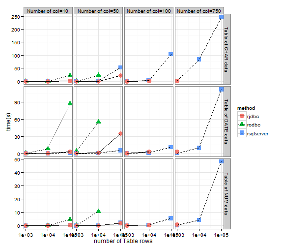
res <- engine(csize == 10 | (csize == 50 & rsize < 1e+05), bencher.table)


res.nordobc <- engine(csize == 50 & rsize == 1e+05 | csize == 100 & rsize <
    1e+05 | csize == 750 & rsize < 10000, bencher.table, remove = "rodbc")

res.nojdbc <- engine(csize == 100 & rsize == 1e+05 | csize == 750 & rsize >=
    10000, bencher.table, remove = c("rodbc", "rjdbc"))

res <- rbind(res.nojdbc, rbind(res, res.nordobc))
ggplot(res, aes(x = rsize, y = time)) + geom_point(aes(color = method, shape = method),
    size = 4) + geom_line(aes(linetype = method)) +
facet_grid(type ~ csize, scales = "free_y", labeller = function(x, y) if (x ==
    "csize") paste0("Number of col=", y) else paste0("Table of ", y, " data")) +

scale_x_log10() + ylab(label = "time(s)") + xlab("number of Table rows")
Since RODBC fails dramatically to extract all rows for big table ( 750 columns with 10^5 rows),
we compare just rsqlserver and rjdbc drivers.

A Typical way to connect to Sql Server from RODBC is to define a Data Source Name or DSN
conn.rodbc <- function() {
    odbcConnect(dsn = "my-dns", uid = "collateral", pwd = "collat")
}
In the other side rsqlserver offer many ways to access to the data base.
You can either specify an url for connection string or specify some parameters like:
- server address
- data base name
- user name and password
One interesting option is to use the Integrated Security and Trusted_Connection arguments. to specify whether the connection is secure, such as Windows Authentication or SSPI. Windows Authentication is sometimes called a trusted connection, because SQL Server trusts the credentials provided by Windows.
So my connection function looks like this:
conn.rsqlserver <- function() {
    url = "Server=localhost;Database=TEST_RSQLSERVER;Trusted_Connection=True;"
    # url = 'Server=localhost;Database=TEST_RSQLSERVER;user
    # id=collateral;password=collat;'
    conn <- dbConnect("SqlServer", url = url)
}
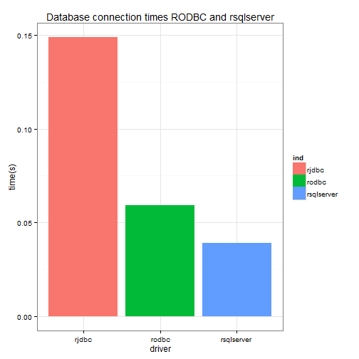
Depending on the application any sub-second response time may be sufficient. But there are many applications where we need a fast data base connection.
conn.rjdbc <- function() {
    drv = JDBC("com.microsoft.sqlserver.jdbc.SQLServerDriver", "d:/temp/sqljdbc_4.0/enu/sqljdbc4.jar")
    url = "jdbc:sqlserver://localhost;user=collateral;password=collat;databasename=TEST_RSQLSERVER;"
    conn <- dbConnect(drv, url = url)
}
tm <- microbenchmark(conn3 <- conn.rjdbc(), conn1 <- conn.rodbc(), conn2 <- conn.rsqlserver(),
times = 1)
dat <- sapply(LIST_DRIVERS, function(driver) microbenchmark:::convert_to_unit(tm[grep(driver,
tm$expr), ]$time, "s"))
ggplot(stack(dat)) + geom_bar(aes(x = ind, y = values, fill = ind), stat = "identity") +
xlab("driver") + ylab("time(s)") + ggtitle("Database connection times RODBC and rsqlserver")
dbBulkCopy is a DBI extension that interfaces the Microsoft SQL Server popular command-line utility named bcp to quickly bulk copying large files into table.
dbBulkCopy extends dbWriteTable and offer best performance an scalability :
- Not limited in number of rows :
dbWriteTablecan write at most 1000 rows. - You can load data from a file or a data.frame. Internally, the data.farme is always saved as a file.
For example a typical use:
- Here I am creating a matrix nrow*ncol
- I save it in a file
- I call dbBulkCopy for quickly bulk copy.
dat <- matrix(round(rnorm(nrow * ncol), 2), nrow = nrow, ncol = ncol)
colnames(dat) <- cnames
id.file = "temp_file.csv"
write.csv(dat, file = id.file, row.names = FALSE)
dbBulkCopy(conn, "NEW_BP_TABLE", value = id.file)