-
Notifications
You must be signed in to change notification settings - Fork 33
Getting started
This tutorial illustrates the basics for using the COMMIT framework to evaluate the evidence of a tractogram.
Important
Commands in this tutorial refer to the latest version of COMMIT. Older versions may not be compatible. The list of changes and updates can be found here.
Download and extract the example dataset from the following ZIP archive, which contains the following files:
-
DWI.nii.gz: a diffusion MRI dataset with 100 measurements distributed on 2 shells, respectively at b=700 s/mm^2 and b=2000 s/mm^2; -
bvals.txtandbvecs.txt: its corresponding acquisition scheme; -
peaks.nii.gz: main diffusion orientations estimated with CSD; -
WM.nii.gz: white-matter mask extracted from an anatomical T1-weighted image.
Also, download the precomputed tractogram from here and put it in the same folder of the extracted data, e.g. demo01_data.
The file demo01_fibers.tck contains about 280K fibers estimated using a streamline-based algorithm.
Open the Python interpreter and go to the folder obtained after extracting the ZIP archive, e.g. demo01_data.
This step precomputes the rotation matrices used internally by COMMIT to create the lookup table for the response functions:
import commit
# commit.setup() # NB: this is required only the first time you run COMMITNow, run the following commands:
from commit import trk2dictionary
trk2dictionary.run(
    filename_tractogram = 'demo01_fibers.tck',
    filename_peaks      = 'peaks.nii.gz',
    filename_mask       = 'WM.nii.gz',
    fiber_shift         = 0.5,
    peaks_use_affine    = True
)
The output should look like this:
Creating data structure from tractogram:
   * Configuration:
      - Segment position = COMPUTE INTERSECTIONS
      - Coordinates shift in X = 0.500 (voxel-size units)
      - Coordinates shift in Y = 0.500 (voxel-size units)
      - Coordinates shift in Z = 0.500 (voxel-size units)
      - Min segment len  = 0.001 mm
      - Min streamline len    = 0.00 mm
      - Max streamline len    = 250.00 mm
      - Do not blur streamlines
      - Output written to "./COMMIT"
      - Temporary files written to "./COMMIT/temp"
      - Using parallel computation with 10 threads
   * Loading data:
      - Tractogram
         - geometry taken from "peaks.nii.gz"
         - 106 x 106 x 60
         - 2.0000 x 2.0000 x 2.0000
         - 283522 streamlines
      - Filtering mask
         - 106 x 106 x 60
         - 2.0000 x 2.0000 x 2.0000
      - EC orientations
         - 106 x 106 x 60 x 9
         - 2.0000 x 2.0000 x 2.0000
         - ignoring peaks < 0.10 * MaxPeak
         - using affine matrix
         - flipping axes : [ x=False, y=False, z=False ]
      - No ISO map specified, using tdi
   * Exporting IC compartments:
      [ 283522 streamlines kept, 15825021 segments in total ]
   * Exporting EC compartments:
      [ 53008 voxels, 145434 segments ]
   * Exporting ISO compartments:
      [ 53008 voxels ]
   * Saving data structure
   * Saving TDI and MASK maps
[ 00:03 ]
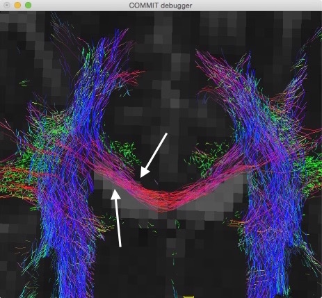
Please note that, in this particular example, in order to have all the data in the same reference system we had to apply a translation of half voxel to the streamlines, as can be noticed in the following figure:

First, we need to convert the bvals/bvecs pair to a single scheme file, using the fsl2scheme function of AMICO:
import amico
amico.util.fsl2scheme( 'bvals.txt', 'bvecs.txt', 'DWI.scheme' )
Now, load the data (see our conventions on the folder structure):
mit = commit.Evaluation()
mit.set_verbose(4)
mit.load_data( 'DWI.nii.gz', 'DWI.scheme' )
Note
The set_verbose(4) set the verbosity level to 4, which is the highest level of verbosity. This tutorial uses this level to show all the details of the fitting process. Without this command, the verbosity level is set to 3 by default, showing the most important information and a progress bar during the fitting process. For more information about the verbosity levels, see here.
The output should be something like:
Loading data:
   * Acquisition scheme:
      - diffusion-weighted signal
      - 100 samples, 2 shells
      - 10 @ b=0, 30 @ b=700.0, 60 @ b=2000.0
   * Signal dataset:
      - dim    : 106 x 106 x 60 x 100
      - pixdim : 2.000 x 2.000 x 2.000
      - values : min=0.00, max=4095.00, mean=54.18
[ 00:00 ]

Preprocessing:
   * Normalizing to b0
      [ min=0.00, max=290.00, mean=0.65 ]
   * Keeping all b0 volume(s)
      [ 106 x 106 x 60 x 100 ]
[ 00:00 ]
For this example we made use of the Stick-Zeppelin-Ball model described in (Panagiotaki et al., NeuroImage, 2012):
- the contributions of the tracts are modeled as "sticks", i.e. tensors with a given axial diffusivity (in this case,
1.7*10^-3 mm^2/s) but null perpendicular diffusivity; - extra-cellular contributions are modeled as tensors with the same axial diffusivity as the sticks and given perpendicular diffusivities (in this case we set only one, i.e.,
0.51^-3 mm^2/s); - isotropic contributions are modeled as tensors with given diffusivities (in this case we set two, i.e.
1.7*10^-3 mm^2/sand3.0*10^-3 mm^2/s).
Setup the parameters of the model and generate the lookup tables:
mit.set_model( 'StickZeppelinBall' )
d_par       = 1.7E-3             # Parallel diffusivity [mm^2/s]
d_perps_zep = [ 0.51E-3 ]        # Perpendicular diffusivity(s) [mm^2/s]
d_isos      = [ 1.7E-3, 3.0E-3 ] # Isotropic diffusivity(s) [mm^2/s]
mit.model.set( d_par, d_perps_zep, d_isos )
mit.generate_kernels( regenerate=True )
mit.load_kernels()
and the output should look like this:
Simulating with "Stick-Zeppelin-Ball" model:
[ 00:00 ]

Loading the kernels:
   * Resampling LUT for subject ".":
      - Keeping all b0 volume(s)
      - Normalizing kernels
[ 00:00 ]
Load in memory the sparse data-structure previously created with trk2dictionary.run():
mit.load_dictionary( 'COMMIT' )The output should show that around 280K streamlines have been loaded, in addition to 145K segments for the extra-cellular contributions in the 53K voxels of the white matter:
Loading the dictionary:
   * Segments from the tracts
      - 283522 fibers and 15825021 segments
   * Segments from the peaks
      - 145434 segments
   * Isotropic contributions
      - 53008 voxels
   * Post-processing
[ 00:02 ]
Now it's time to build the linear operator A which computes the matrix-vector multiplications for solving the linear system. This operator uses information from the segments loaded in the previous step and the lookup tables for the response functions; it also splits the workload to different threads (if possible) during the multiplications. To this aim, run the following commands:
mit.set_threads()
mit.build_operator()
The output should be similar to this:
Distributing workload to different threads:
   * Number of threads : 10
   * A operator
   * A' operator
[ 00:01 ]

Building linear operator A:
[ 00:02 ]
Note
The number of threads is automatically set to the maximum number found in the system (4 in this example), but this value can be manually set, e.g., mit.set_threads( 1 ).
To fit the model (Stick-Zeppelin-Ball in this case) to the data, simply run:
mit.fit( tol_fun=1e-3, max_iter=1000 )In order to solve the NNLS problem, before starting the fit, the regularisation is set to None and the non negativity constraint is used.
Setting regularisation:
   * IC compartment:
      - Non-negativity constraint: True
   * EC compartment:
      - Non-negativity constraint: True
   * ISO compartment:
      - Non-negativity constraint: True
[ 00:00 ]

Fit model:

      |  1/2||Ax-y||^2      Omega      |  Cost function    Abs error      Rel error    |      Abs x          Rel x
------|--------------------------------|-----------------------------------------------|------------------------------
   1  |  2.8815304e+05  0.0000000e+00  |  2.8815304e+05  4.0316380e+05  1.3991308e+00  |  5.4060948e+01  1.0000000e+00
   2  |  2.3368418e+05  0.0000000e+00  |  2.3368418e+05  5.4468867e+04  2.3308753e-01  |  1.6252137e+01  2.6646384e-01
   3  |  1.9736251e+05  0.0000000e+00  |  1.9736251e+05  3.6321671e+04  1.8403532e-01  |  1.4524594e+01  2.0468222e-01
...
...
 138  |  1.0236157e+04  0.0000000e+00  |  1.0236157e+04  1.0582135e+01  1.0337996e-03  |  1.5259300e+00  4.0981471e-03
 139  |  1.0225869e+04  0.0000000e+00  |  1.0225869e+04  1.0288392e+01  1.0061142e-03  |  1.5166781e+00  4.0656073e-03
 140  |  1.0215874e+04  0.0000000e+00  |  1.0215874e+04  9.9943213e+00  9.7831286e-04  |  1.5070904e+00  4.0323663e-03
< Stopping criterion: Relative tolerance on the objective >
[ 00:20 ]
where the columns report, among other information, the iteration number, the current cost function and its relative change between two consecutive iterations.
The estimated streamline weights, i.e., streamline_weights.txt, and the voxelwise output maps, i.e., fit_RMSE.nii.gz, can be stored to files as follows:
mit.save_results()As shown in the output, the results are saved in the folder Results_StickZeppelinBall:
Saving results to "Results_StickZeppelinBall/*":
   * Fitting errors:
      - RMSE:  0.059 +/- 0.018
      - NRMSE: 0.118 +/- 0.037
   * Voxelwise contributions:
      - Intra-axonal
      - Extra-axonal
      - Isotropic
   * Configuration and results:
      - streamline_weights.txt
      - results.pickle
[ 00:00 ]
The streamline weights estimated by COMMIT, i.e., one coefficient for each streamline in the input tractogram demo01_fibers.tck, can be found in the file streamline_weights.txt:
0.00000e+00
0.00000e+00
0.00000e+00
0.00000e+00
1.47401e-03
3.36807e-03
2.32047e-03
1.02605e-05
8.35506e-06
0.00000e+00
...
...
If you need the estimated coefficients for all the compartments, you can access these values with:
x_ic, x_ec, x_iso = mit.get_coeffs()
print( x_ic.size ) # this shows there are 283522 streamline coefficients (one for each)
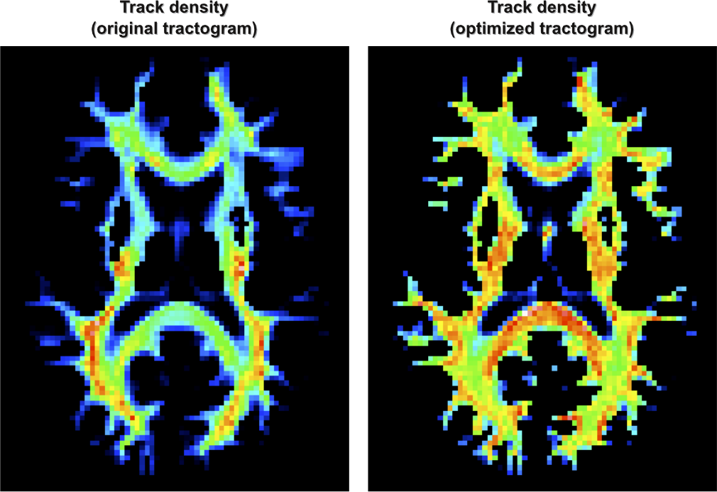
The following figure shows the density of the tracts (Calamante et al., NeuroImage, 2010) of the original tractogram (left) and of its optimized version (right):

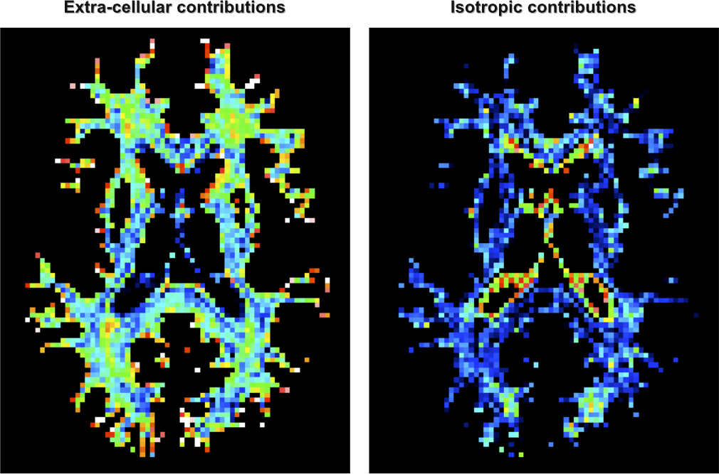
It is also possible to visualize voxelwise maps of the corresponding contributions of the extra-cellular space (left) and other isotropic contaminations (right):

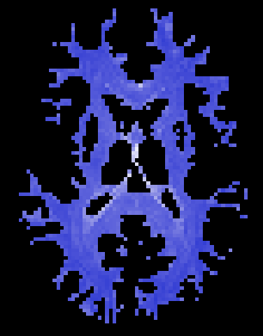
Finally, the fitting error in each voxel can also be inspected:

 Diffusion Imaging and Connectivity Estimation (DICE) lab