LatticeGrid

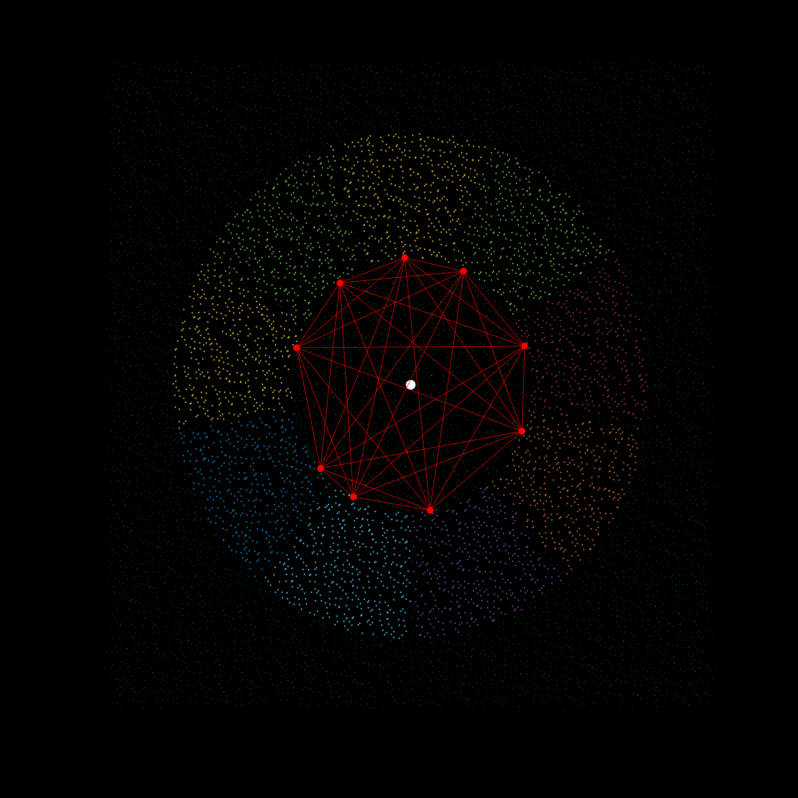
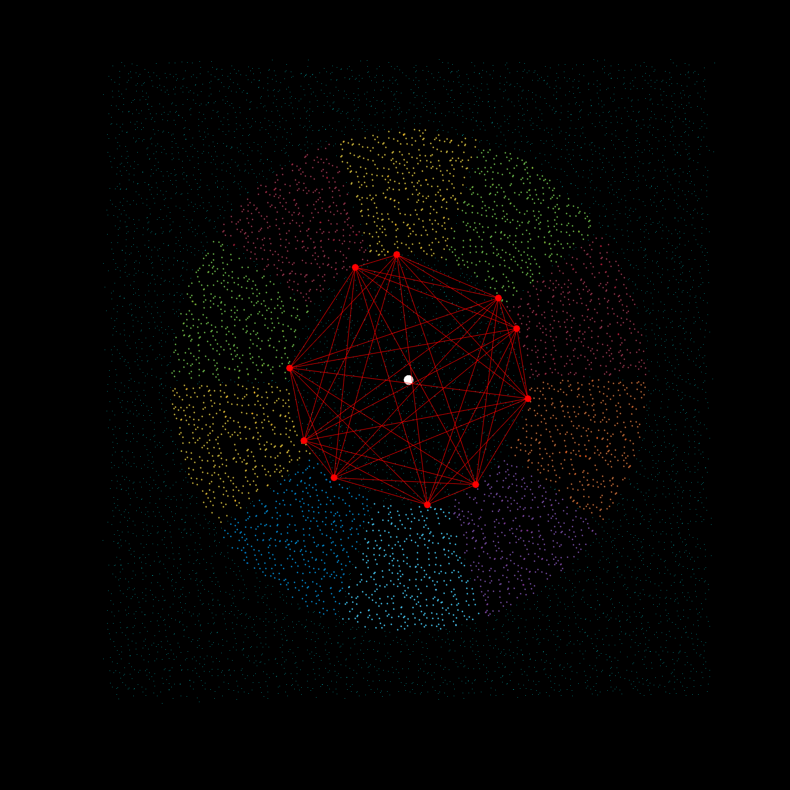
This is Matlab code that describes a method to smooth raw scattered surface data into a regular lattice. Datasets from scans, such as Sonar and LIDAR data, often are segmented into several sections, and each datapoint is irregularly scattered across the surface. Formalizing several different datasets into a single lattice surface allows for feature visualization and analysis without the compromise of irregularly scattered data that can bias results. The six steps shown here describe a novel method.

Lattice vs Mosaic

Step 1

Load and compile your 3D raw data (fine if datasets spatially overlap), here called Basin, and isolate each spatial dimension into its X, Y, and Z vectors. Extract the maximum and minimum values of each vector using the nanmax and nanmin functions, these six values (two per vector) are the three-dimensional edges of the complete dataset.

X=Basin(:,1);Xmin=nanmin(X);Xmax=nanmax(X);
Y=Basin(:,2);Ymin=nanmin(Y);Ymax=nanmax(Y);
Z=Basin(:,3);Zmin=nanmin(Z);Zmax=nanmax(Z);

Step 2

The following two steps are deceitfully simple: the goal is to create a regular lattice from the known edges. First we make regularly spaced points between the edges of the X and Y dimensions, calling the new regularized vectors Xi and Yi. Then an empty vector filled with ones of length Yi is created as a placeholder for the next step. The reciprocal of the step number is used as the determinant of length, but I haven't figured out an elegant way to connect the final vector lengths of Xi and Yi with code. The specific numbers shown here (0.5479999999:1 ratio) come from manual trial and error. It has to do with Matlab using an index starting at 1 instead of 0, but it works!

step=24999;
Xi=(Xmin:1/step:Xmax)';
Yi=(Ymin:0.5479999999/step:Ymax)';
string=length(Yi);
newOne=ones(string,1);

Step 3

This for-loop populates the newOne vector and turns it into a periodic newX vector for every X position in the new lattice. Simultaneously, each iteration adds a new newY value, looping across Y positions until a new X position is required. This creates an XY grid bound within the nanmax and nanmin limits of X and Y.

for i=1:string
    if i==1
        stanzaX=Xi(i,1);
        newX=newOne.*stanzaX;
        stanzaY=Yi;
        newY=stanzaY;
    else
        stanzaX=Xi(i,1);
        longX=newOne.*stanzaX;
        newX=cat(1,newX,longX);
        stanzaY=Yi;
        newY=cat(1,newY,stanzaY);
    end
end

Step 4

Creating the point cloud ptCloud, a placeholder object with all the original X and Y information and a zero dummy vector to be populated by the Z dimension, or the vector newZ.

xyzPoints=cat(2,X,Y,zeros(length(Z),1));
ptCloud=pointCloud(xyzPoints);
newZ=zeros(length(newX),1);

Step 5

In this step everything comes together. The vector newZ gets populated by elevation data from the original X and Y data now in ptCloud using a k-nearest neighbor algorithm, here using the two closest points from the cloud and averaging them to populate the respective newZ point. This is repeated millions of times, so a modulo of every 1000000th iteration prints the i number to check progress. This step takes about 2 hours to complete, depending on how large the datasets are.

for i=1:1:length(newX)
    b=mod(i,1000000);
    	if b==0
   	i
    	end
    point=[newX(i,:),newY(i,:),0];
    K=2;
    [indices,dists]=findNearestNeighbors(ptCloud,point,K);
    pickZ=Z(indices);
    pointZ=nanmean(pickZ);
    newZ(i,1)=pointZ;
end

Step 6

Exporting into vectors, and into a final 3D vector, here called XYZ_Basin.

XYZ_Basin=cat(3,newX,newY,newZ);

This can be exported as a .csv file (or .xyz file) for visualizations in graphical engine software.

Kernel for k-nearest search

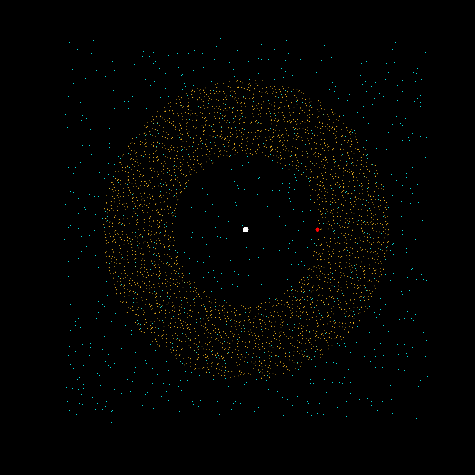
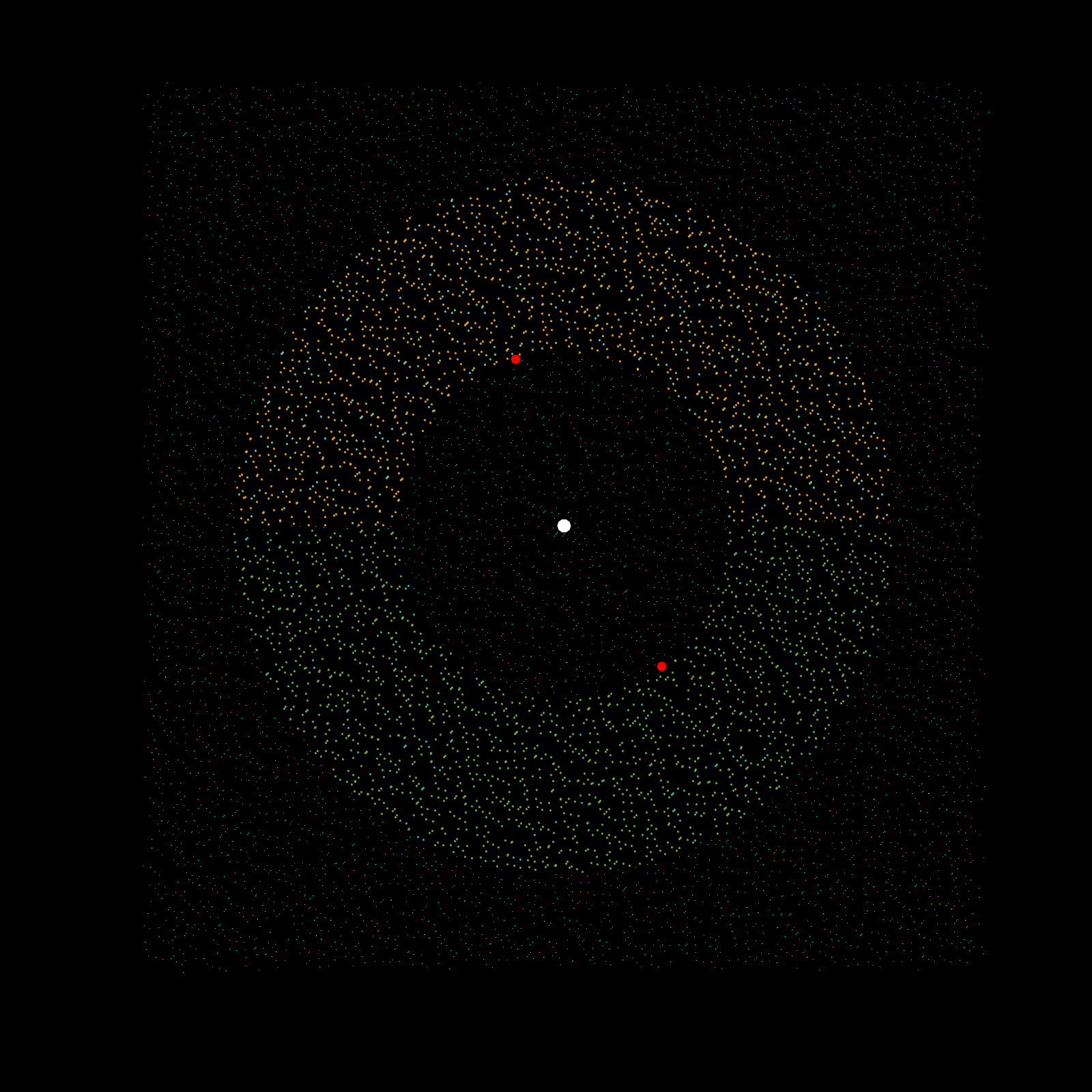
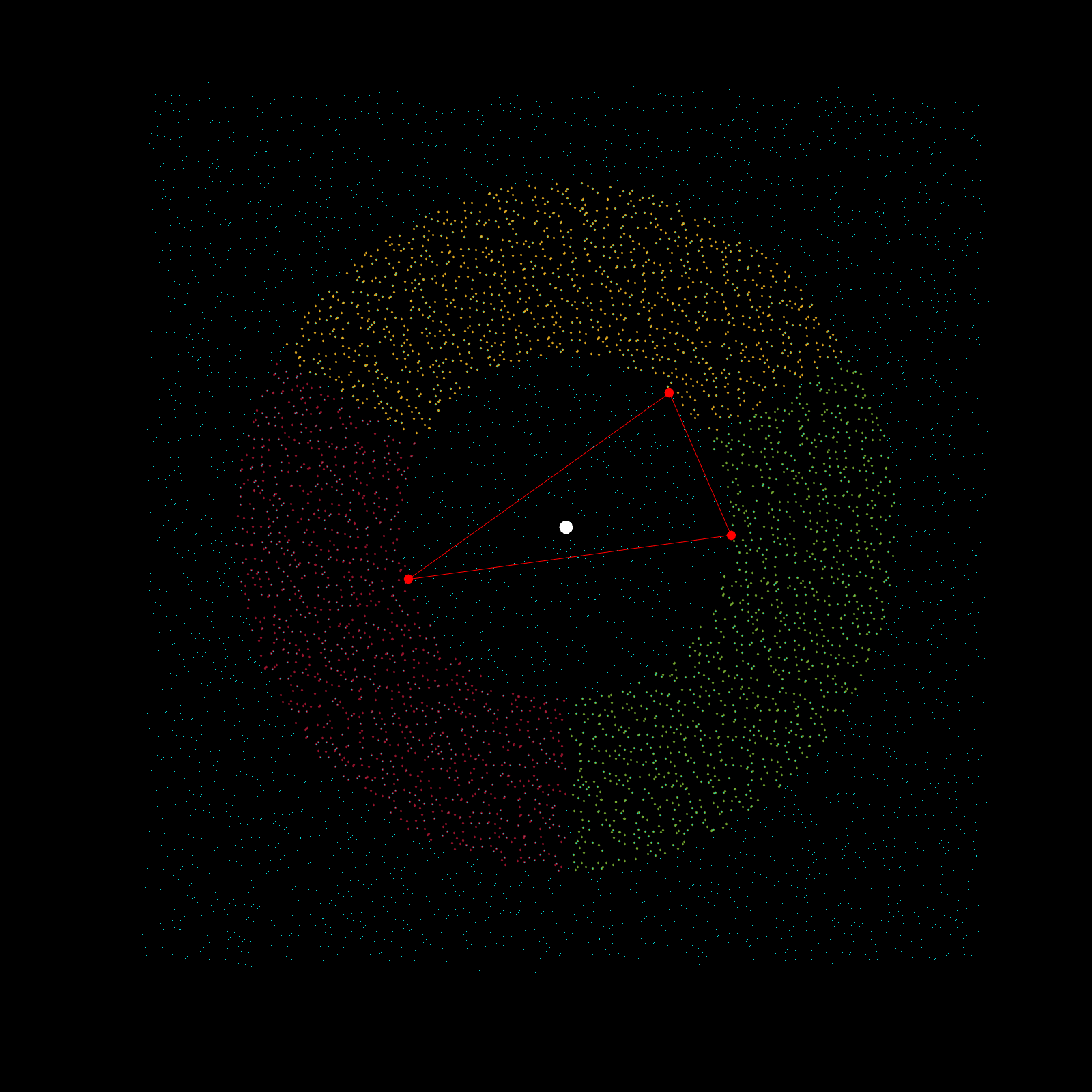
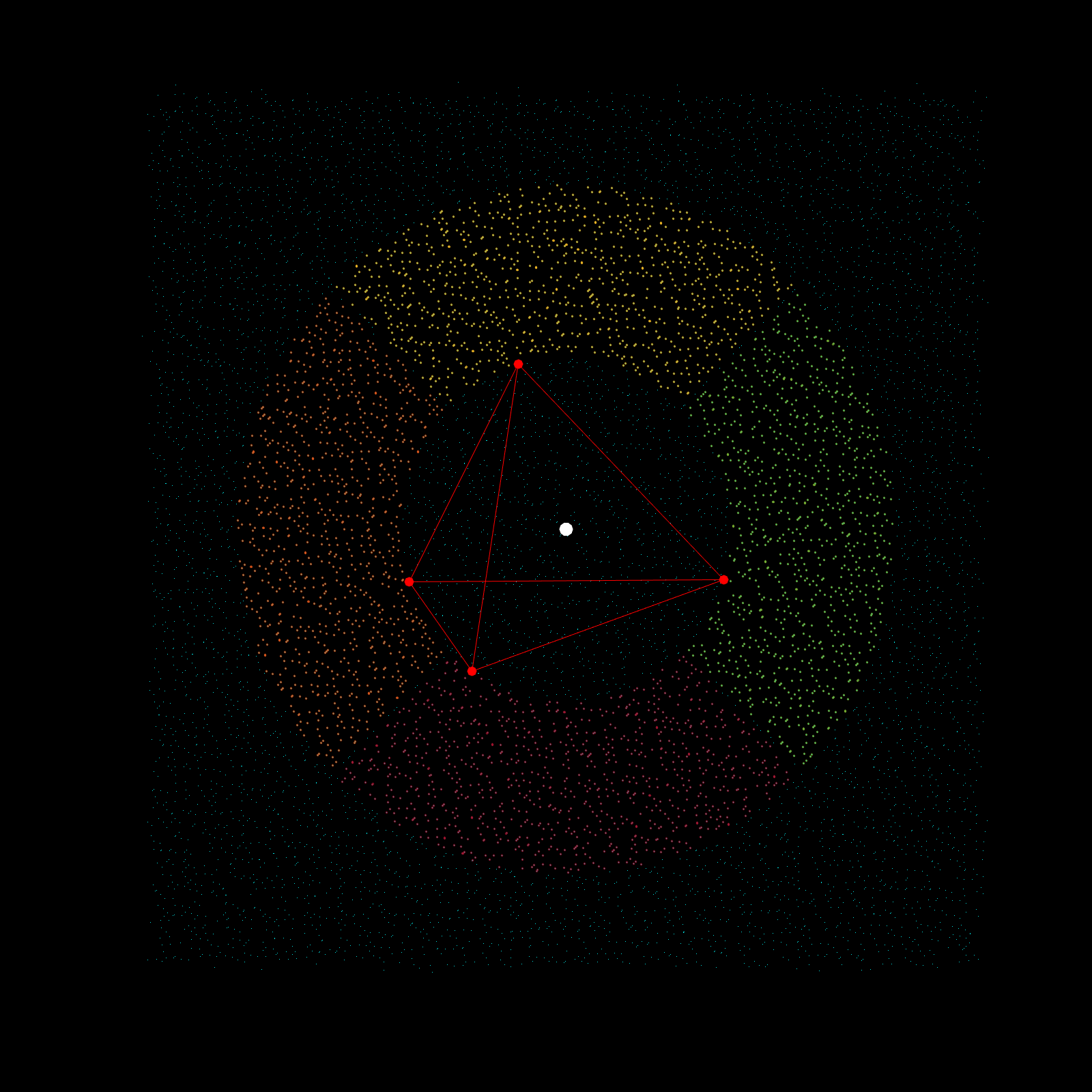
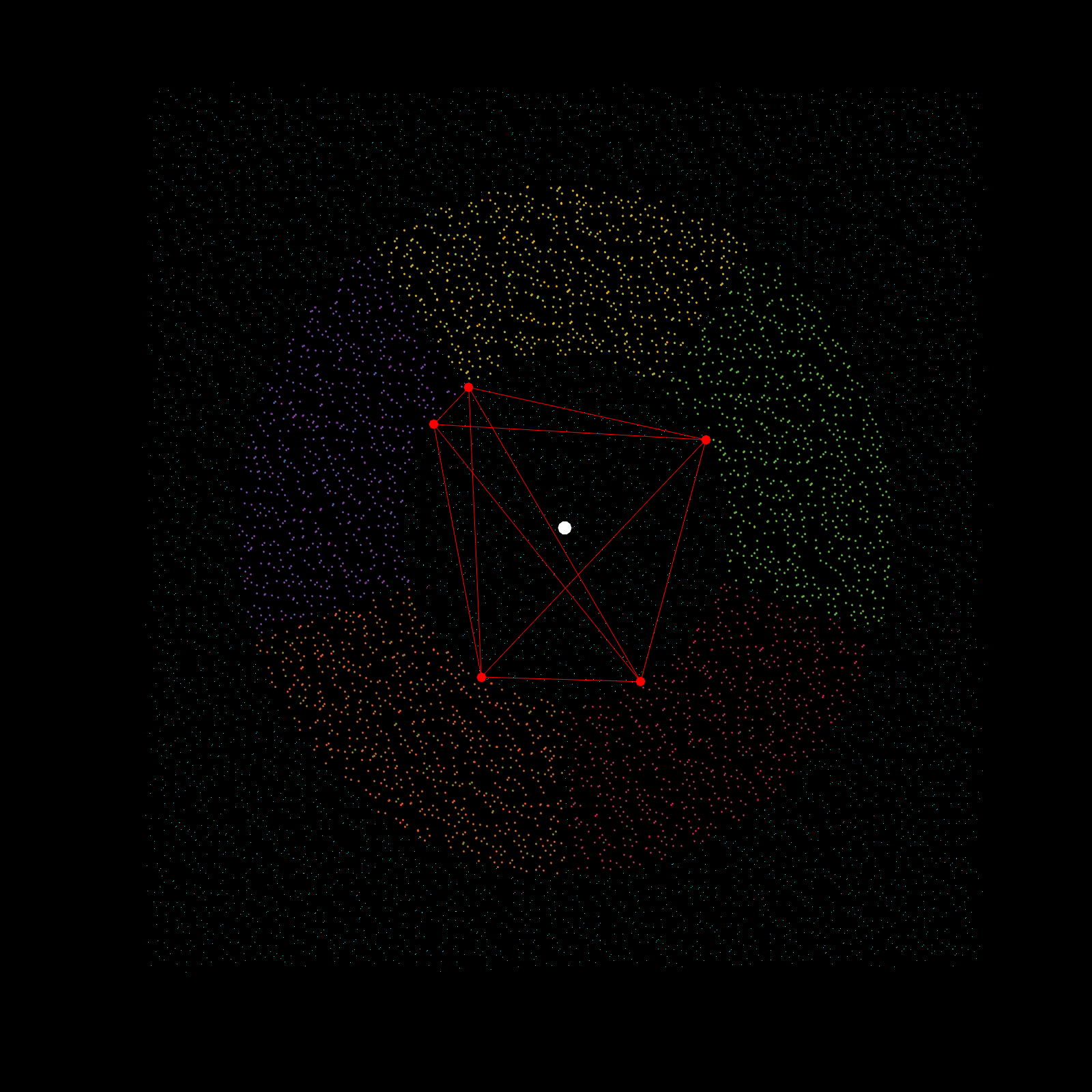
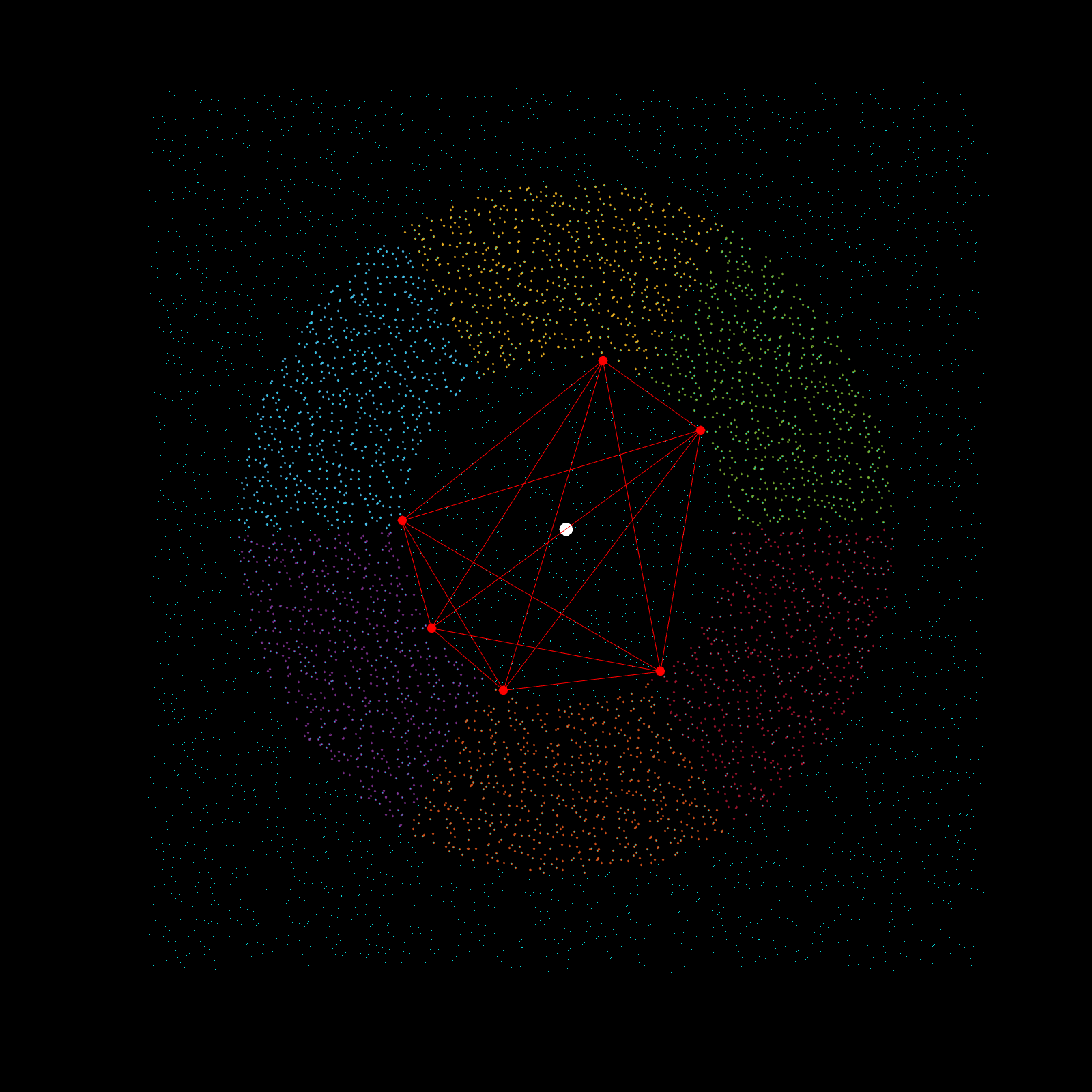
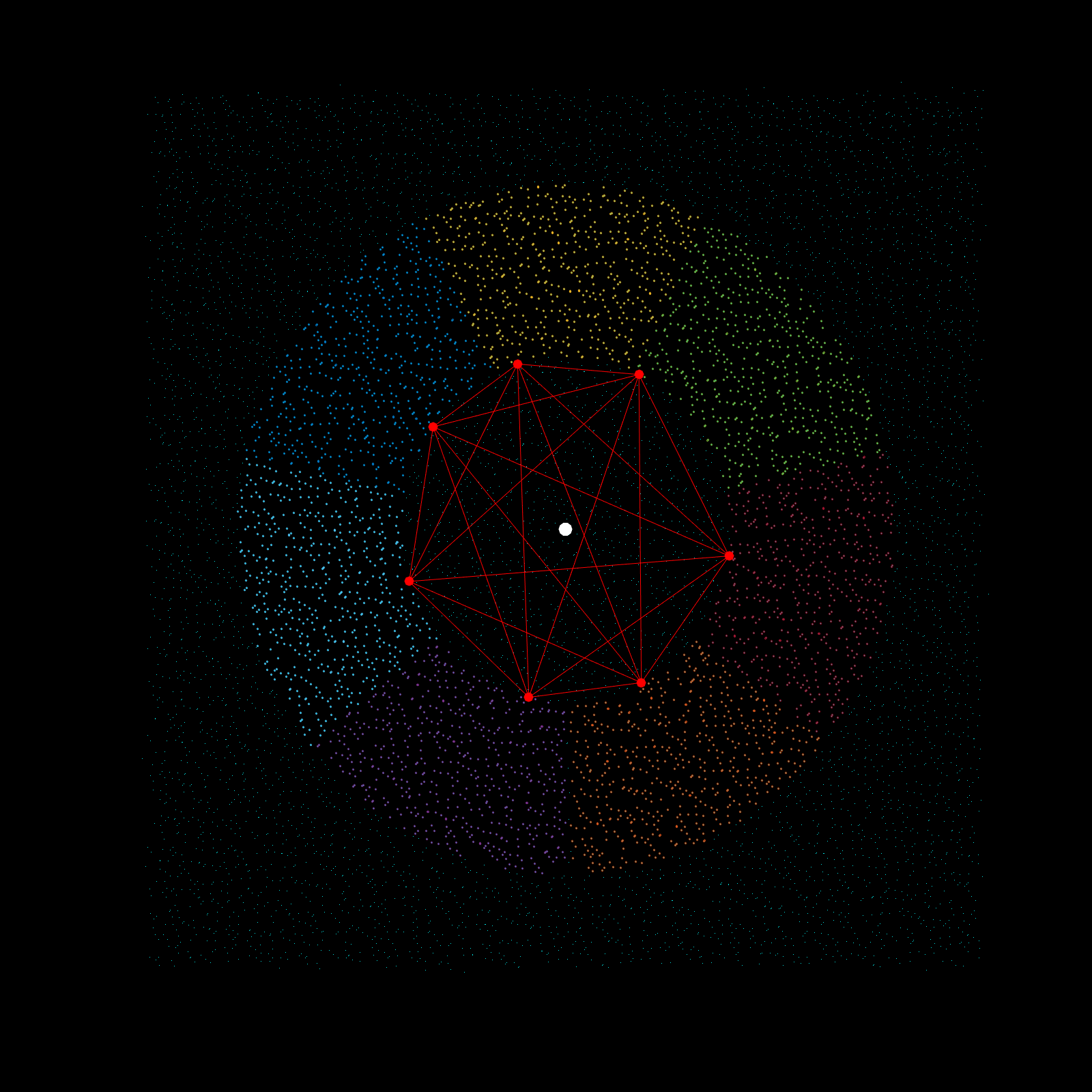
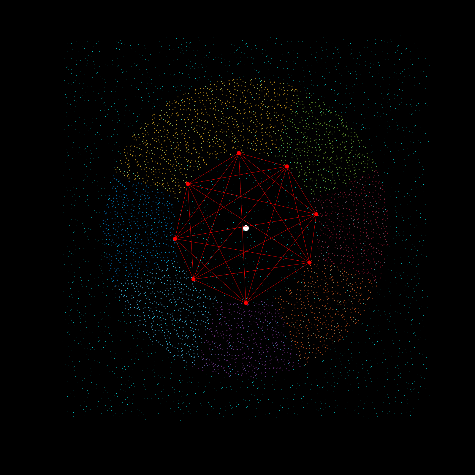
Imagine a gigantic chess board and a king piece. In this analogy the model lattice is the board, and the kernel is the king piece. The piece moves one square at a time, linearly, till each column is sweeped, and then moving to the next column, until every chess tile is visited once. This is the basic architecture of how a uniform lattice elevation model is created from a mosaic of eclectic datasets. The kernel size k determines how many “neighboring” tiles the king gathers information from, in turn used to assign an average elevation to the visited tile in that iteration. A large k is smoothing because it collapses many neighboring tiles into a single value (convolution), whereas a small k produces a sharper (but more jagged) surface, since it averages a smaller region. Kernel size also determines its shape, which in this case is in the shape of a simplex. A simplex is a polytope that extends into an arbitrary number of dimensions. Described here is the code to visualize n-sided simplex.

simplex=[3;4;5;6;7;8;9;10];
 
poly=nsidedpoly(simplex);
Z=rescale(rand([simplex,1]),-1,1);
X=poly.Vertices(:,1);
Y=poly.Vertices(:,2);
Kernel=cat(2,X,Y,Z);
 
Xa=[];Ya=[];Za=[];
Xb=[];Yb=[];Zb=[];
 
figure('Position',[650,10,780,780],'Resize','off','Color','k');hold on;
set(gca,'CameraViewAngleMode','manual');axis off;axis equal;
scatter3(Kernel(:,1),Kernel(:,2),Kernel(:,3),0.01,'w','filled');
scatter3(0,0,0,500,'w','filled');
 
count=0;colors=(plasma(length(Kernel)));
 
for i=1:length(Kernel)
    A=Kernel(i,:);
    for q=1:length(Kernel)
        if q>=i
        else
            count=count+1;
            B=Kernel(q,:);
            Xa(count)=A(1,1);Ya(count)=A(1,2);Za(count)=A(1,3);
            Xb(count)=B(1,1);Yb(count)=B(1,2);Zb(count)=B(1,3);
            plot3([A(1,1);B(1,1)],[A(1,2);B(1,2)],[A(1,3);B(1,3)],'-', ...
            'Color',colors(i,:),'LineWidth',1);
            drawnow;pause(0.05);
        end
    end
end

Advanced kernel with angle-forced k-nearest search

Using the same k value as the seed for the simplex, the advanced kernel creates a k-sided regular polygon that slices the mosaic data in radial regions, and then performs k-nearest search once per region. This guarantees the simplex, which indeed does arise from noisy mosaic data, is also selecting from all cardinal points for its Z-value calculation. This creates phenomenal smoothing, best interpolation results yet!