
Skin cancer is the most prevalent type of cancer. Melanoma, specifically, is responsible for 75% of skin cancer deaths, despite being the least common skin cancer. In this project we aim to analyze and identify melanoma in lesion images. Current disease diagnosis based on human labor is not only time-consuming but may prove to be inefficient as well. This endeavor of ours aims to leverage the potential of Computer Vision and Machine Learning to to successfully categorize the given melanoma image into malignant or benign.
Melanoma is a deadly disease, but if caught early, most melanomas can be cured with minor surgery. Image analysis tools that automate the diagnosis of melanoma will improve dermatologists' diagnostic accuracy. Better detection of melanoma has the opportunity to positively impact millions of people.
This project was a part of 'SIIM-ISIC Melanoma Classification' challenge hosted on Kaggle.
Read more at : https://www.kaggle.com/c/siim-isic-melanoma-classification
The dataset was generated by the International Skin Imaging Collaboration (ISIC) and images are from the following sources: Hospital Clínic de Barcelona, Medical University of Vienna, Memorial Sloan Kettering Cancer Center, Melanoma Institute Australia, The University of Queensland, and the University of Athens Medical School. A copy of the dataset was made available on Kaggle platform and may also be located on ISIC 2020 challenge webpage. The links are pasted below :
- The ISIC 2020 Challenge Dataset : https://challenge2020.isic-archive.com/
- Kaggle : https://www.kaggle.com/c/siim-isic-melanoma-classification/data
The dataset was made available under Creative Commons Attribution-Non Commercial 4.0 International License.
It encapsulated :
- Images in DICOM, jpeg and TFRecord format.
- 33,126 training images were provided along with 10,982 test images.
- Each image belonged to either of the two categories : malignant or benign.
Some randomly sampled images from the training set :


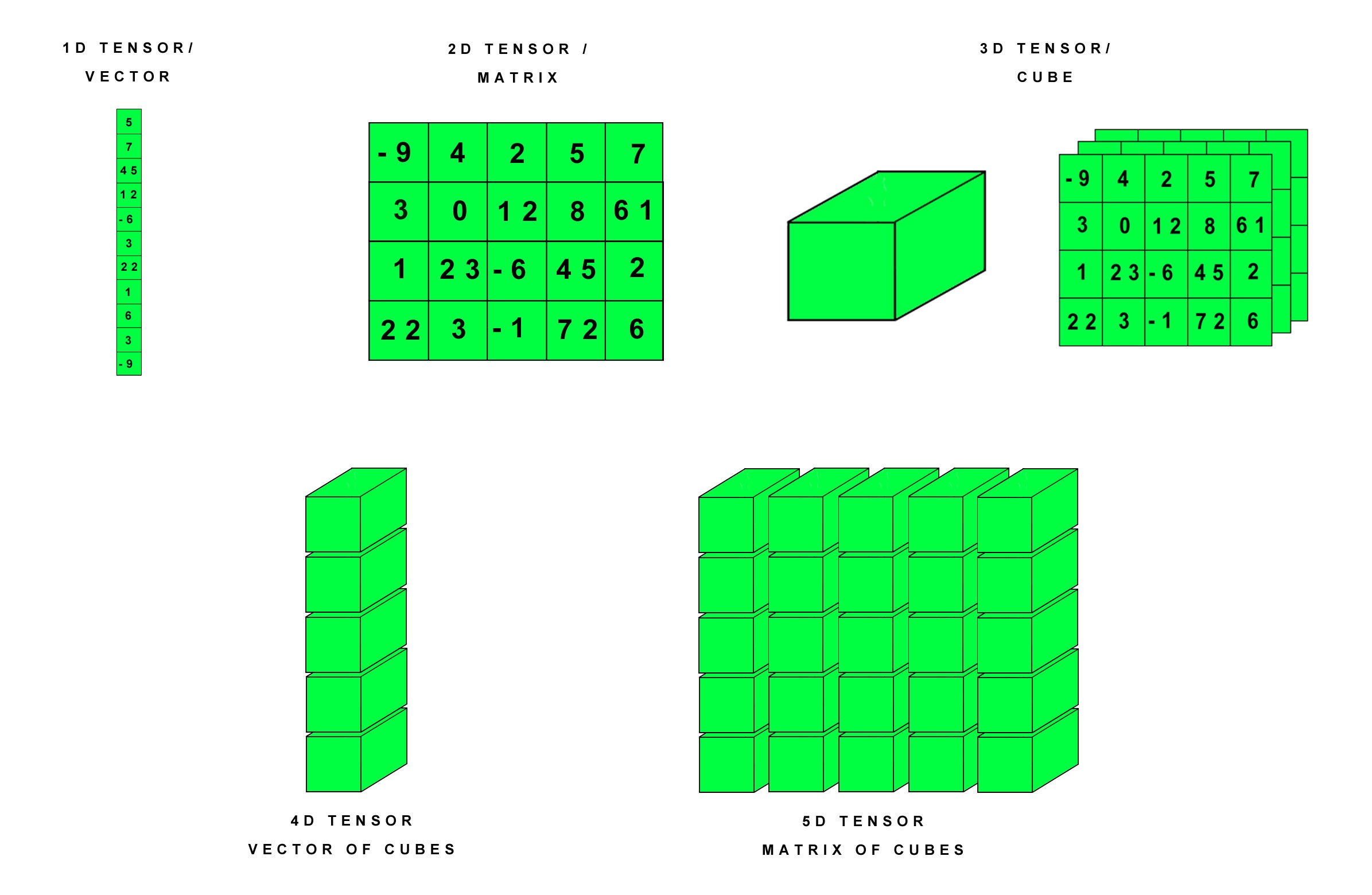
- Numpy : Fundamental package for scientific computing in Python3, helping us in creating and managing n-dimensional tensors. A vector can be regarded as a 1-D tensor, matrix as 2-D, and so on.
- Pandas : Pandas is a software library written for the Python programming language for data manipulation and analysis. In particular, it offers data structures and operations for manipulating numerical tables and time series.

- Matplotlib and Seaborn : Python3 plotting libraries used for data visualization.

- OpenCV : OpenCV (Open Source Computer Vision Library) is an open source computer vision and machine learning software library. OpenCV was built to provide a common infrastructure for computer vision applications and to accelerate the use of machine perception in the commercial products. The library has more than 2500 optimized algorithms, which includes a comprehensive set of both classic and state-of-the-art computer vision and machine learning algorithms. The library is used extensively in companies, research groups and by governmental bodies.
Homepage : https://opencv.org/

- Tensorflow : Is an open source deep learning framework for dataflow and differentiable programming. It’s created and maintained by Google.

- SciKit-Learn : Scikit-learn is a free software machine learning library for the Python programming language. It features various classification, regression and clustering algorithms.

- tqdm : Is a progress bar library with good support for nested loops and Jupyter notebooks.
In order to avoid unnecessary computation during the Exploratory Data Analysis(EDA) that follows, here we will prepare custom dataframe encapsulating necessary image oriented features such as :
- Image Name
- Image Path
- Number of Rows
- Number of Columns
- Channels
- Image Mean
- Image Standard Deviation
- Image Skewness
- Mean Red Value
- Mean Green Value
- Mean Blue Value
The notebook is also available on Kaggle : https://www.kaggle.com/fireheart7/melanoma-a-story-in-3-parts-part-one?scriptVersionId=38737538
Notebook link(code is also available in this repository) : https://www.kaggle.com/fireheart7/melanoma-a-story-in-3-parts-part-two
When we’re getting started with a machine learning (ML) project, one critical principle to keep in mind is that data is everything. It is often said that if ML is the rocket engine, then the fuel is the (high-quality) data fed to ML algorithms. However, deriving truth and insight from a pile of data can be a complicated and error-prone job. To have a solid start for our ML project, it always helps to analyze the data up front.
During EDA, it’s important that we get a deep understanding of:
- The properties of the data, such as schema and statistical properties;
- The quality of the data, like missing values and inconsistent data types;
- The predictive power of the data, such as correlation of features against target.
Upon loading and inspecting the dataframes for train and test, we found :
Train Insights :

Test Insights :

- Training set : Sex, age and anatomy_site have missing values.
- Test set : Anatomy_site have missing values.
We also found that out of 33,126 registered entries in the training set, only 2,056 are unique implying that some patients are diagnosed with multiple marks. Same goes for the test set where we have only 690 unique values out of collection of 10,982.
The following snapshots will say it all!!
Benign VS Malignant Overall :

Male VS Female Counts :

Malignant Male Cases VS Female Cases :

Benign Male VS Female Cases :

Cancer VS Sex :

Age VS Cancer :

Anatomy Sites :

Probablistic Age Distribution In Training Set :

Spread of Red Channel in BENIGN CASES :

Spread Of Green Channel in BENIGN CASES :

Spread Of Blue Channel in BENIGN CASES :

So,
Spread In Benign :

Spread In Malignant :

So, we observe that in both the cases the component of red spikes the most, whereas Blue and Green are close to each other. All the channels also appears to be a bit negatively skewed.
Hence, the channel distribution won't be a powerful feature to differentiate between the malignant and benign cases.
Kutosis of this distribution is manageable.
Anatomy sites, patient's sex and age values were previously found missing which were then filled here according to the insights obtained in the EDA before. Read the notebook or the code file. Markdowns are provided for the logic used to decide how to fill the missing values.


We observe that most common dimension in training and testing set's intersection is 1800 X 1800 to 2500 X 2500.
In the end, we analyze image mean,standard deviation and skewness with one another. For this we will use plotly's express. Plotly Express is the easy-to-use, high-level interface to Plotly, which operates on a variety of types of data and produces easy-to-style figures.
Train Images 3-D Analysis :

Test Images 3-D Analysis :

For this project we worked using TFRecords, which is binary storage format for our data.

The binary storage data takes up relatively low space on our disk, and hence it takes less time to copy and can be read much more efficiently! Moreover, the tensorflow framework is optimized to handle tfrecords amazingly well.
The datasets that are too large to be stored fully in memory, this is an advantage as only the data that is required at the time (e.g. a batch) is loaded from disk and then processed.
Another major advantage of TFRecords is that it is possible to store sequence data — for instance, a time series or word encodings — in a way that allows for very efficient and (from a coding perspective) convenient import of this type of data.
A TFRecord file contains an array of Examples. Example is a data structure for representing a record, like an observation in a training or test dataset. A record is represented as a set of features, each of which has a name and can be an array of bytes, floats, or 64-bit integers.
To summarize:
- An Example contains Features.
- Features is a mapping from the feature names stored as strings to Features.
These relations are defined in example.proto and feature.proto in the TensorFlow's source code, along with extensive comments. As the extension .proto suggests, these definitions are based on protocol buffers.

Google’s Protocol buffers are a serialization scheme for structured data. In other words, protocol buffers are used for serializing structured data into a byte array, so that they can be sent over the network or stored as a file. In this sense, it is similar to JSON, XML.
Protocol buffers can offer a lot faster processing speed compared to text-based formats like JSON or XML.
The aforemntioned TFRecords are crunched using TPU which we initialized in our code.
TPUs are hardware accelerators specialized in deep learning tasks. We used the one provided by Kaggle platform for this project.

Each TPU core has a traditional vector processing part (VPU) as well as dedicated matrix multiplication hardware capable of processing 128x128 matrices. This is the part that specifically accelerates machine learning workloads.
TPUs are equipped with 128GB of high-speed memory allowing larger batches, larger models and also larger training inputs.
The tf.data API enables us to build complex input pipelines from simple, reusable pieces and use the resources to a superlative degree of efficiency. Hence, these effective data pipelines ensures that our accelerator TPU/GPU is always crunching and stays idle for a minimum time span.
The following will illustrate the advantage of an efficient pipeline design :

Before procedding further, a batch encapsulated in TFRecord is viewed to ensure the I/O design successfully works :

Upon inspection, the malignant to benign ratio was found to be 0.017. This denotes extreme skewness about the dataset(as exposed in the EDA as well) that is much needed to be addressed. So, malignant cases are assigned a higher class weight compared to the benign ones. This will encourage the model to pay more attention to malignant ones.
According to official Tensorflow documentation :
Optional dictionary mapping class indices (integers) to a weight (float) value, used for weighting the loss function (during training only). This can be useful to tell the model to "pay more attention" to samples from an under-represented class.
A callback is a powerful tool to customize the behavior of a Keras model during training, evaluation, or inference. Callbacks are useful to get a view on internal states and statistics of the model during training.
This can be used to stop predictions when there is no change in the desired metric over a certain epoch range. This is amazingly useful in order to avoid overfitting.
When we compile our model, we do not want our metric to be accuracy. If we run the model, with an accuracy metric, it will give us false confidence in our model. If we look at the dataset, we see that 98% of the images are classifed as benign, 0. Now, if accuracy was the sole determinant of our model, a model that always outputs 0 will achieve a high accuracy although the model is not good.
We will use ROC Curve to evaluate, which is why our metric will be set to tf.keras.metrics.AUC.

For this a custom head was designed to fit onto the head of the pre-trained imported model. Various architectures were tried, such as ResNet50, EfficientNet, DenseNet, however from the point of view of production, we settled on MobileNetV2 Architecture as it only has a 2-3 million parameters. This architecture can be effectively deployed in production, and also it gave us an overall accuracy of about 85% on the test set and 86% on the training set.
The training result :

All these notebooks have also been published on Kaggle :
- TFRecord Design : https://www.kaggle.com/fireheart7/melanoma-design-tf-records
- Melanoma - A Story in Three Parts- Part One : https://www.kaggle.com/fireheart7/melanoma-a-story-in-3-parts-part-one
- Melanoma - A Story in Three Parts - Part Two : https://www.kaggle.com/fireheart7/melanoma-a-story-in-3-parts-part-two
- Melanoma - A Story in Three Parts - Part Three : https://github.com/CodingWitcher/SIIM-ISIC-Melanoma-Classification/blob/master/MobileNetV2.ipynb (This repository)
Thank you for reading this far!!
Contact : bauraiaditya7@gmail.com