-
Notifications
You must be signed in to change notification settings - Fork 2
Statistical Inference
UA DATALAB WORKSHOP SERIES
📓 These notes: https://github.com/ua-datalab/Workshops/wiki/Statistical-Inference/
💻 Codebase with examples: Statistical_Inference.ipynb

(Image credit: Florian Geiser, Towards AI Medium)
Exploratory Data Analysis (EDA) is an important first step in data analysis.
Here are some key points:
- Data Exploration: EDA involves summarizing the main characteristics of a dataset, such as data distribution and central tendencies (mean, median) and spread (variance, standard deviation).
John Tukey promoted the five-number summary is a set of descriptive statistics that provides information about a dataset.
(Figure: Boxplot example)
It consists of the five most important sample percentiles:
- the sample minimum (smallest observation)
- the lower quartile or first quartile
- the median (the middle value)
- the upper quartile or third quartile
- the sample maximum (largest observation)
-
Data Visualization: Visualizations like histograms, box plots, scatter plots, and correlation matrices are used to represent data patterns and relationships. Visualization aids in identifying outliers, trends, and potential insights
-
Data Cleaning: EDA often includes handling missing values, outliers, and inconsistencies to ensure reliable data.
-
Univariate Analysis: This step focuses on analyzing individual variables, including summary statistics and visualizations.
-
Bivariate Analysis: EDA examines relationships between pairs of variables to uncover associations.
-
Identifying Patterns: EDA aims to find patterns, trends, or anomalies in the data.
-
Hypothesis Generation: EDA can generate initial hypotheses or research questions.
-
Communication: EDA results are presented visually and effectively communicated to stakeholders.
Overall, EDA helps understand the structure and content of a dataset, guiding subsequent analysis techniques.

Seaborn is a Python library for statistical data visualization. It is designed to work seamlessly with pandas DataFrames and is built on top of Matplotlib, making it a powerful tool for creating attractive and informative statistical graphics.
Here are key points about Seaborn:
Statistical Visualization: Seaborn specializes in creating statistical visualizations. It provides a high-level interface for drawing informative and attractive statistical graphics.
Integration with Pandas: Seaborn works well with pandas DataFrames, allowing you to easily visualize data stored in pandas structures.
Built on Matplotlib: Seaborn utilizes Matplotlib underneath for plotting, which means you can customize and fine-tune your plots using Matplotlib functions if needed.
Default Styles and Palettes: Seaborn comes with beautiful default styles and color palettes, making it effortless to create visually appealing plots.
Widely Used in Data Science: It is commonly used in data science and machine learning tasks for visualizing data distributions, relationships, and patterns.
For reading and cleaning data, as well as for doing data analysis, the Pandas Python Library is the preferred choice for every day data science tasks. Pandas also includes a set of essential visualization functions to explore the dataset properties.
We will present a small collection of open source software Python tools that will facilitate us carrying out an Exploratory Data Analysis of a dataset with a small amount of coding necessary.
Statistical inference in data science refers to the process of drawing conclusions or making predictions about a population based on a sample of data. It plays a crucial role in extracting meaningful insights from data.
Here are key points to understand about statistical inference:
-
Sample to Population: Statistical inference involves extrapolating insights from a sample dataset to make statements about the larger population it represents. It addresses questions like, "What can we infer about the entire population based on this sample?"
-
Types of Statistical Inference: There are two main types of statistical inference:
-
Descriptive Statistics: This aspect involves summarizing and describing data using measures like mean, median, and standard deviation, but it doesn't make predictions or inferences about the population.
-
Inferential Statistics: This includes hypothesis testing, confidence intervals, regression analysis, and more. It aims to make predictions, test hypotheses, and draw conclusions about the population.
-
-
Procedure: Statistical inference typically involves several steps, including data collection, hypothesis formulation, statistical analysis, and drawing conclusions.
-
Importance in Data Science: Statistical inference is fundamental in data science as it allows data scientists to make data-driven decisions, test hypotheses, and assess the significance of results.
Statistical inference is a cornerstone of data science, enabling professionals to extract meaningful insights and make informed choices from data.
When working with statistics within Python, several essential packages are commonly used for data analysis and statistical modeling:
- Scipy.stats. This module contains a large number of probability distributions, summary and frequency statistics, correlation functions and statistical tests, masked statistics, kernel density estimation, quasi-Monte Carlo functionality, and more.
- Pandas: tabular data, time series functionality, interfaces to other statistical languages.
- Pingouin: open-source statistical based mostly on Pandas and NumPy.
- statsmodels: regression, linear models, time series analysis, extensions to topics also covered by scipy.stats.
- PyMC: Bayesian statistical modeling, probabilistic machine learning.
- Seaborn: statistical data visualization.

Statsmodels is a Python package that plays a crucial role in statistical modeling and analysis. It offers a wide range of functionalities for estimating various statistical models and conducting statistical analysis.
Here's a concise overview of Statsmodels:
Statistical Modeling: Statsmodels provides classes and functions for estimating diverse statistical models. These models encompass linear and non-linear regression, generalized linear models, time-series analysis, and more.
Statistical Testing: It includes advanced functions for statistical testing. This is essential for hypothesis testing, assessing model fit, and making statistical inferences from data.
Data Exploration: Statsmodels facilitates statistical data exploration. You can use it to explore the relationships between variables, visualize data, and gain insights into the underlying statistical properties.
Complement to SciPy: While SciPy offers a foundation for scientific computing, Statsmodels complements it by focusing on statistical computations. It's particularly useful for researchers, data scientists, and statisticians.
Statsmodels is a valuable tool for anyone working with data analysis and statistical modeling in Python. You can find detailed documentation and examples on the official Statsmodels website.
In probability theory and statistics, a probability distribution is the mathematical function that gives the probabilities of occurrence of different possible outcomes for an experiment. It is a mathematical description of a random phenomenon in terms of its sample space and the probabilities of events.
You can find a long list of probability distributions here. Some of these distribution functions are important in several applications, so they have their own names.
Here, we will address only a small set of them.

The general form of its probability density function is
The parameter
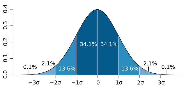
The Central Limit Theorem tells us that the sum of many independent and identically distributed variables approximates a normal distribution. These distributions are characterized by a mean and standard deviation, and everything from human height, IQ scores, and even the velocities of gas molecules follow a normal distribution (See more examples)

In probability theory, a log-normal (or lognormal) distribution is a continuous probability distribution of a random variable whose logarithm is normally distributed. Thus, if the random variable X is log-normally distributed, then Y = ln(X) has a normal distribution.
The probability distribution function for the log-normal distribution is
The distribution of financial assets, or particle sizes generated by grinding, blood pressure and metabolic rates in various organisms usually follow a log-normal distribution.
The log-normal distribution often arises from multiplicative growth processes, in which it is repeatedly multiplied by some random factor.

The Exponential distribution is often used to model the time between events in a Poisson process. The probability density function (PDF) for the Exponential distribution is given by:
The exponential distribution is a continuous probability distribution that often concerns the amount of time until some specific event happens. It is a process in which events happen continuously and independently at a constant average rate.
Example of this type of process is the radioactive decay of certain chemical elements, or the time (starting now) until an earthquake occurs, or the time until a device fails (See more examples)
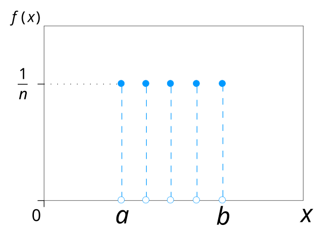
The discrete uniform distribution is a symmetric probability distribution where a finite number of equally likely outcomes are observed, with each outcome having a probability of 1/n.
The probability distribution function is

All outcomes have the same probability. In the continuous case, the probability density function is flat between the minimum and maximum values. Rolling a fair die or choosing a card from a well-shuffled deck follows uniform distributions (See more examples).

In probability theory and statistics, the Poisson distribution is a discrete probability distribution that expresses the probability of a given number of events occurring in a fixed interval of time or space if these events occur with a known constant mean rate and independently of the time since the last event.
The Poisson distribution models the number of times a radioactive atom decays in a given period, or the number of cars that pass a given point in a given time. If an average of 10 cars pass per minute at an intersection, the Poisson distribution can estimate the probability that 15 cars pass in the next minute. Similarly, in sports such as hockey or soccer, where goals are infrequent, the distribution can be used to model the number of goals scored by each team (See more examples).

Binomial distribution is a probability distribution that summarizes the likelihood that a variable will take one of two independent values under a given set of parameters. The distribution is obtained by performing a number of Bernoulli trials.
A Bernoulli trial is assumed to meet each of these criteria :
-
There must be only 2 possible outcomes.
-
Each outcome has a fixed probability of occurring. A success has the probability of
$p$ , and a failure has the probability of$1 – p$ . -
Each trial is completely independent of all others.
The probability mass function (PMF) for a Binomial distribution is given by:
for
The binomial random variable represents the number of successes(r) in n successive independent trials of a Bernoulli experiment (See more examples).
📓 See Jupyter Notebook Example
Every probability distribution can be described in an alternate way using a Moment-generating function. This function is an infinite series, each term of this is called a moment.
The first moment is the expected moment (a.k.a. arithmetic mean), the second central moment is the variance, the third standardized moment is the skewness, the fourth moment is the kurtosis, and so on...
import numpy as np
import scipy.stats as ss

### Specify Data
n  = 10000
m1 = 0
m2 = 1
# m3 =
# m4 =

### Generate synthetic data (Normal distribution)

x = np.random.normal(m1, m2, n)

# Compute the first four moments

M1 = np.mean(x)
M2 = np.var(x)
M3 = ss.skew(x)
M4 = ss.kurtosis(x)
The next table summarizes the relationships between the distribution function parameters and their first four moments.
| Distribution | mean: M1 | variance: M2 | skewness: M3 | Excess kurtosis: M4 |
|---|---|---|---|---|
| Normal | 0 | 0 | ||
| Exponential | 2 | 6 | ||
| Uniform | 0 | |||
| Poisson | ||||
| Binomial |
- Probability & Statistics resources, C. Lizárraga, UArizona Data Lab.
- Probability & Statistics Cheat Sheet. Afshine Amidi & Shervine Amidi.
- Understanding Probability Distributions using Python | Jupyter Notebook. Reza Bagheri.
- Machine Learning Foundations | Probability & Information | Statistics. Jon Krohn.
Created: 10-04-2023 (C. Lizárraga); Updated: 02-06-2024 (C. Lizárraga)
UArizona DataLab, Data Science Institute, University of Arizona, 2024.
UArizona DataLab, Data Science Institute, University of Arizona, 2024.

