personal reference repository for common algorithms and data structures implementation
-
Big O notation does not determine the actual execution time of an algorithm, but rather provides a way to classify algorithms based on their scalability.
-
It provides an upper bound on the time complexity of an algorithm, indicating how the algorithm's execution time grows as the size of the input increases.
what is Big-O Notation and what is Omega and Theta ?
-
Big-O Notation(worst case) is a mathematical Notation used to describe the limiting behavior of a function when the argument tends towards a particular value or infinity.
It is commonly used in computer science to describe the time complexity of algorithms.-
Big-O Notation Mathematical exepression
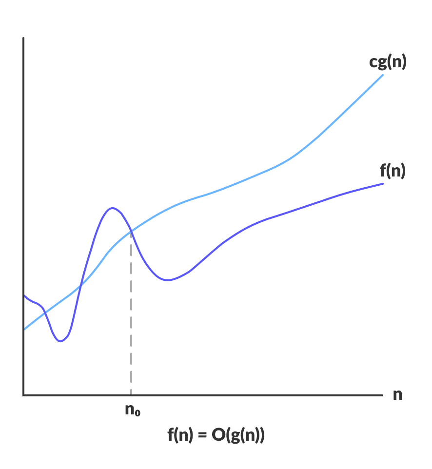
O(g(n)) = { f(n): there exist positive constants c and n0 such that 0 ≤ f(n) ≤ cg(n) for all n ≥ n0 }
-
Big-O Notation Graph
-
-
Omega Notation (best case) , on the other hand, provides a lower bound on the running time of an algorithm. It is used to describe the best-case running time of an algorithm.
-
Omega Notation Mathematical exepression
Ω(g(n)) = { f(n): there exist positive constants c and n0 such that 0 ≤ cg(n) ≤ f(n) for all n ≥ n0 }
-
-
Theta Notation(both O(g(n)) and Ω(g(n))) is used to describe the tight bound on the running time of an algorithm. It provides both an upper and a lower bound on the running time of an algorithm. In other words, if a function is Θ(g(n)), then it is both O(g(n)) and Ω(g(n)).
-
Theta Notation Mathematical exepression
Θ(g(n)) = { f(n): there exist positive constants c1, c2 and n0 such that 0 ≤ c1g(n) ≤ f(n) ≤ c2g(n) for all n ≥ n0 }
-
-
Big-O Notation measures the upper bound or worst-case scenario for the growth rate of a function. In the context of computer science and algorithm analysis, it is used to describe the maximum amount of time an algorithm takes to solve a problem as the input size grows.
-
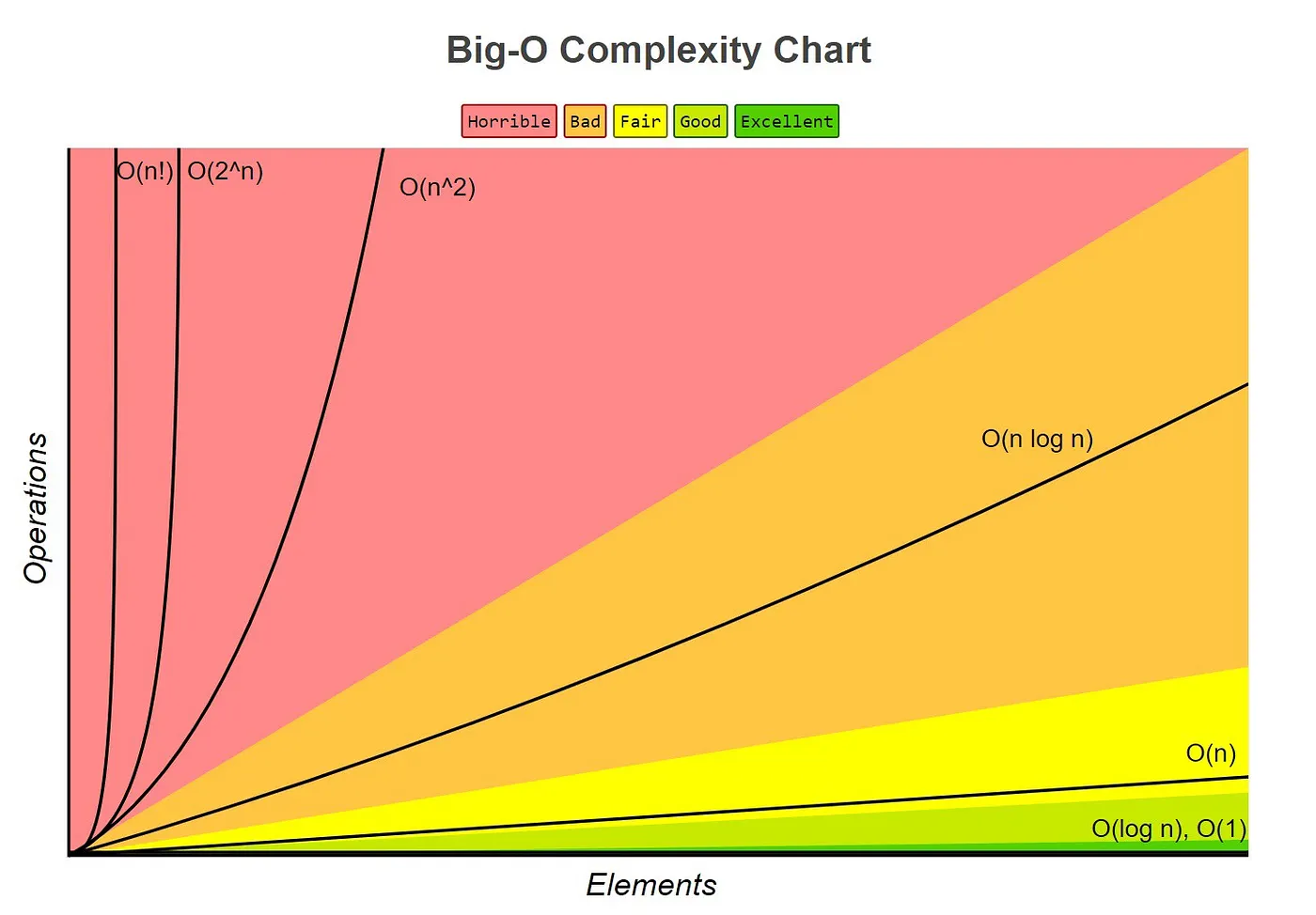
Big-O Complexity Chart
- Big O notation does not determine the actual execution time of an algorithm, but rather provides a way to classify algorithms based on their scalability.
-
It provides an upper bound on the time complexity of an algorithm, indicating how the algorithm's execution time grows as the size of the input increases.
-
Static Array: Contiguous area of memory consisting of equal-size elements indexed by contiguous integers.
- Read / Write Time Complexity
- Access: O(1)
- Add/Remove (start / middle): O(n)
- Add/Remove (end): O(1)
- Read / Write Time Complexity
-
Dynamic Array: A dynamic array is an array with a big improvement: automatic resizing.
-
Problem: Static arrays are fixed in size, meaning they're not able to expand or contract once they're created. This is a problem for two reasons:
-
- We might insert items and then run out of capacity.
-
- We might delete items and end up with lots of empty space at the end of the array.
-
-
Solution: dynamic arrays (also known as resizable arrays)
-
Idea: store pointer to a dynamically allocated array and replace it with a newly-allocated array as needed.
- Unlike static arrays, dynamic arrays can be resized.
- Appending an item to a dynamic array is O(1) on average, but O(n) worst-case, because of the possibility of having to allocate a new array and copy over the old elements.
- Some space is wasted the capacity is always at least the length of the array, but usually, it's somewhere between length and length * 2.
- is a linear data structure, in which the elements are not stored at contiguous memory locations. The elements in a linked list are linked using pointers.
- data structure for storing objects in a linear fashion. It is a collection of nodes where each node holds a node value and a link to the next node in the list.
- Advantages:
- Dynamic size
- Ease of insertion/deletion
- Disadvantages:
- Random access is not allowed. We have to access elements sequentially starting from the first node. So we cannot do binary search with linked lists efficiently with its default implementation.
- Extra memory space for a pointer is required with each element of the list.
- Not cache friendly. Since array elements are contiguous locations, there is locality of reference which is not there in case of linked lists.
- Use Cases:
- Linked lists are used to implement stacks, queues, graphs, etc.
- dynamic memory allocation
| Array | Linked List | |
|---|---|---|
| Order determined by | indices | pointers |
| Search | O(1) | O(n) |
-
The order of the elements in an array is determined by their indices. For example, if we have an array of integers {1, 2, 3, 4}, then the first element is at index 0, the second element is at index 1, and so on.
-
The order of the elements in a linked list is determined by the pointers that connect the nodes together. For example, if we have a linked list with three nodes containing the data values 1, 2, and 3, then the order of the elements is determined by the pointers connecting the nodes: node 1 points to node 2, which points to node 3.
-
Singly Linked Lists: is a data structure that contains a sequence of nodes such that each node contains an object and a reference to the next node in the list.
-
Doubly Linked Lists: is a data structure that contains a sequence of nodes such that each node contains an object and references to the previous and next nodes in the list.
-
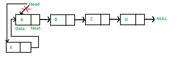
Circular Linked Lists: is a variation of a linked list in which the last element is linked to the first element. This forms a circular loop.
- Unlike arrays, linked list elements are not stored at contiguous locations; the elements are linked using pointers.
- Accessing an element in a linked list is a linear operation because we have to sequentially traverse the list until we find the desired element.
- Linked lists have dynamic size, unlike arrays which have fixed size. So, it is not required to pre-allocate memory for a linked list.
- The drawbacks of using linked list are that they require extra memory for pointers and they are not cache friendly (elements are not stored in contiguous locations).
-
A Stack is a collection of objects that are inserted and removed according to the last-in, first-out (LIFO) principle.
-
- push: O(1)
- pop: O(1)
- top: O(1)
-
- Backtracking
- finding the correct path in a maze
- Undo
- undoing an action in a word processor
- Call Stack
- keeping track of function calls in a program
- depth-first search
- keeping track of visited nodes in a graph or tree
- Backtracking
-
I used Dynamic Array & Linked List to implement Stack.
-
A Queue is a collection of objects that are inserted and removed according to the first-in, first-out (FIFO) principle.
-
- enqueue: O(1)
- dequeue: O(1)
- front: O(1)
-
-
Customer service call centers: When a customer calls a support line, their call is put in a queue until a representative is available to take their call. The representative will then take the calls in the order they were received.
-
Printers: When multiple documents are sent to a printer, they are placed in a queue and processed one at a time. The first document to be sent to the printer is the first one to be printed, and the subsequent documents are printed in the order they were received.
-
Operating systems: When a program requests memory from the operating system, the operating system will place the program in a queue and allocate memory to the program when memory becomes available.
-
Breadth-first search: When searching a tree or graph, we can use a queue to store the nodes that we have yet to visit. The nodes are placed in a queue in the order they are visited, and removed from the queue in the same order.
-
-
I used Dynamic Array & Linked List to implement Queue.
- A Hash Table is a data structure that maps keys to values for highly efficient lookup.
- Indexing in databases
- Cryptography
- Symbol Tables in Compilers
- Dictionary, caches, etc
- Insert: O(1)
- Delete: O(1)
- Search: O(1)
-
Direct Access Table
- If we want a data structure to store a set of integers, we can use an array to store the value at an index equal to the integer. For example, if we want to store the set of integers {1, 4, 5, 8, 10}, we can create an array of size 11 (the largest integer in the set plus one) and store the value at the index equal to the integer. The value at index 0 will be unused, and the value at index 1 will be 1, the value at index 4 will be 4, and so on. This data structure is called a direct-access table because we can directly access the values in the array using the integers as indices.
- keys may not be non negative integers
- gigantic memory hog
-
Solution for 1
- prehashing (
hash(x)in python) ==> maps keys to non negative integers hash(x)use the default id, which is the physical location of the object in memory- (no to items occupy the same memory location)
- prehashing (
-
Solution for 2
-
hashing: what we talked about before going into this simple approach
-
reduce universal of all keys down to reasonable size m for table
-
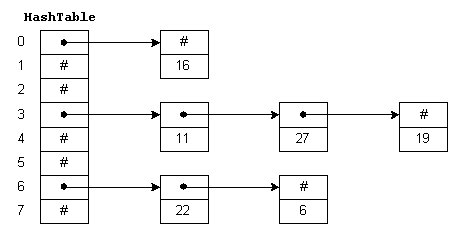
there in the last image: h(k2) == h(k5) which is a collision
-
if we assume that n is the number of keys and m is the size of the table the average number of keys in each linked list is n/m so the average time complexity of searching is O(1 + (n/m)) keep in mind that if the n is much smaller than m the average time complexity is O(1) but we will have a lot of empty space in the table and if the n is much bigger than m the average time complexity is O(n)
- so we want m to be big enough to avoid collision and small enough to avoid empty space-
so How to choose m?
- first approach is to choose m to be some small constant let's say 8 and we extend the table and shrink it when needed BUT thhis approach is comming with the previous concept of dynamic array Amortization
-
- collision: two distinct keys map to the same slot in the hash table
-
Hashing with chaining is a method of collision resolution In this method we use a linked list to store the collided keys
-
probing: try to see if we can insert something into the hash table, and if you fail, we're going to recompute a slightly different hash function and try again
insert(key, value): keep probing until an empty slot is found. Once an empty slot is found, insert key.search(key): keep probing until slot’s key doesn’t become equal to given key or an empty slot is reached.delete(key): delete operation is interesting. If we simply delete a key, then search may fail. So slots of deleted keys are marked specially as “deleted”.
- in this method we use the next empty slot in the table to store the collided key according to the following formula
h(key,i) = (h'(key) + i) mod mwhere h'(key) is an ordinary hashing function
and i is the number of collisions
and m is the size of the table
and h(key,i) is the probing function
- disadvantage of this method is **clustering**
the problem with the clusters is that it will grow rapidly for example if we have a table of size 100 and we have a cluster of 4 items in the table and we want to insert a new item the probability of collision is 4/100 = 4% which is 4 time bigger than the probability of collision in the first place and we can essentially argue through making probabilistic assumptions that that if in fact we use linear probing we will lose our avg. constant time lookup
- MIT OPEN COURSEWARE
- in this method we use the next empty slot in the table to store the collided key according to the following formula
h(key,i) = (h'(key) + i*h''(key)) mod mwhere h'(key) is an ordinary hashing function
and h''(key) is another hashing function
and i is the number of collisions
and m is the size of the table
-
Division method
in this method we divide the key by the size of the table and take the remainder
def hash(key, size):
    return key % size
-
Multiplication method
key = [a*k mod 2^w] >> (w-r)
in this method we multiply the key by a constant a and take the most significant bits
where a is a random number between 0 and 2^w
and r is the number of bits we want to take (m = 2^r)
and w is the number of bits in word in the machinedef hash(key, size): a = random.randint(0, 2**w) return ((a*key) % 2**w) >> (w-r)
-
Universal hashing
key = (a*k + b) mod p mod m
in this method we multiply the key by a constant a and add another constant b and take the remainder
where a and b are random numbers between 0 and p
p is a huge prime number (bigger than the size of key universe)
m is the size of the tabledef hash(key, size): p = "HUGE PRIME NUMBER" a = random.randint(0, p) b = random.randint(0, p) return ((a*key) + b) % p % size
this method is better than the previous methods because it's more random
and if the a,b randomization is done correctly it will be very hard to find a collision
the Pr of collision is 1/m


