All have been tested with python2.7+ and tensorflow1.0+ in linux.

• Samples: save generated data, each folder contains a figure to show the results.
• utils: contains 2 files
  • data.py: prepreocessing data.
  • nets.py: Generator and Discriminator are saved here.

For research purpose,
Network architecture: all GANs used the same network architecture(the Discriminator of EBGAN and BEGAN are the combination of traditional D and G)
Learning rate: all initialized by 1e-4 and decayed by a factor of 2 each 5000 epoches (Maybe it is unfair for some GANs, but the influences are small, so I ignored)
Dataset: celebA cropped with 128 and resized to 64, users should copy all celebA images to ./Datas/celebA for training

• DCGAN
• EBGAN
• WGAN
• BEGAN
  And for comparsion, I added VAE here.
• VAE

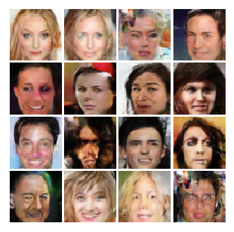
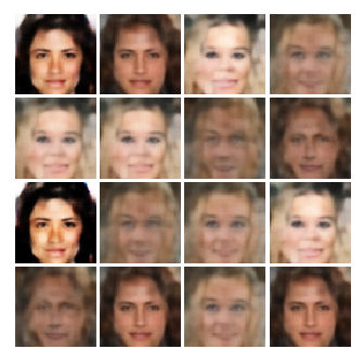
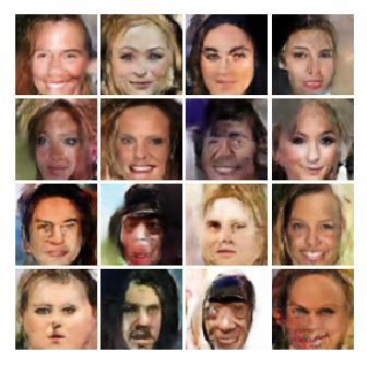
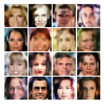
The generated results are shown in the end of this page.

---

Theories

✨DCGAN

Main idea: Techniques(of architecture) to stabilize GAN
Unsupervised Representation Learning with Deep Convolutional Generative Adversarial Networks[2015]

Loss Function (the same as Vanilla GAN)

Architecture guidelines for stable Deep Convolutional GANs

• Replace any pooling layers with strided convolutions (discriminator) and fractional-strided convolutions (generator).
• Use batchnorm in both the generator and the discriminator
• Remove fully connected hidden layers for deeper architectures. Just use average pooling at the end.
• Use ReLU activation in generator for all layers except for the output, which uses Tanh.
• Use LeakyReLU activation in the discriminator for all layers.

---

✨EBGAN

Main idea: Views the discriminator as an energy function Energy-based Generative Adversarial Network[2016]
(Here introduce EBGAN just for BEGAN, they use the same network structure)

What is energy function?

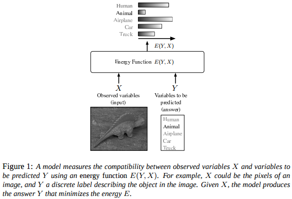
The figure is from LeCun, Yann, et al. "A tutorial on energy-based learning."

In EBGAN, we want the Discriminator to distinguish the real images and the generated(fake) images. How? A simple idea is to set X as the real image and Y as the reconstructed image, and then minimize the energy of X and Y. So we need a auto-encoder to get Y from X, and a measure to calcuate the energy (here are MSE, so simple).
Finally we get the structure of Discriminator as shown below.

So the task of D is to minimize the MSE of real image and the corresponding reconstructed image, and maximize the MSE of fake image from the G and the corresponding reconstructed fake image. And G is to do the adversarial task: minimize the MSE of fake images...
Then obviously the loss function can be written as:

And for comparison with BEGAN, we can set the D only as the auto-encoder and L(*) for the MSE loss. Loss Function

m is a positive margin here, when L(G(z)) is close to zero, the L_D is L(x) + m, which means to train D more heavily, and on the contrary, when L(G(z))>m, the L_D is L(x), which means the the D loosens the judgement of the fake images.

Finally, there is a quetion for EBGAN, why use auto-encoder in D instead of the traditonal one? What are the benifits?
I have not read the paper carefully, but one reason I think is that (said in the paper) auto-encoders have the ability to learn an energy manifold without supervision or negative examples. So, rather than simply judge the real or fake of images, the new D can catch the primary distribution of data then distinguish them. And the generated result shown in EBGAN also illustrated that(my understanding): the generated images of celebA from dcgan can hardly distinguish the face and the complex background, but the images from EBGAN focus more heavily on generating faces.

---

✨Wasserstein GAN

Main idea: Stabilize the training by using Wasserstein-1 distance instead of Jenson-Shannon(JS) divergence
GAN before using JS divergence has the problem of non-overlapping, leading to mode collapse and convergence difficulty.
Use EM distance or Wasserstein-1 distance, so GAN can solve the two problems above without particular architecture (like dcgan).
Wasserstein GAN[2017]

Mathmatics Analysis
Why JS divergence has problems? pleas see Towards Principled Methods for Training Generative Adversarial Networks

Anyway, this highlights the fact that the KL, JS, and TV distances are not sensible cost functions when learning distributions supported by low dimensional manifolds.

so the author use Wasserstein distance

Apparently, the G is to maximize the distance, while the D is to minimize the distance.

However, it is difficult to directly calculate the original formula, ||f||_L<=1 is hard to express. So the authors change it to the clip of varibales in D after some mathematical analysis, then the Wasserstein distance version of GAN loss function can be: Loss Function

Algorithm guidelines for stable GANs

• No log in the loss. The output of D is no longer a probability, hence we do not apply sigmoid at the output of D

	G_loss = -tf.reduce_mean(D_fake)
	D_loss = tf.reduce_mean(D_fake) - tf.reduce_mean(D_real) 

• Clip the weight of D (0.01)

	self.clip_D = [var.assign(tf.clip_by_value(var, -0.01, 0.01)) for var in self.discriminator.vars]

• Train D more than G (5:1)
• Use RMSProp instead of ADAM
• Lower learning rate (0.00005)

---

✨ BEGAN

Main idea: Match auto-encoder loss distributions using a loss derived from the Wasserstein distance
BEGAN: Boundary Equilibrium Generative Adversarial Networks[2017]

Mathmatics Analysis
We have already introduced the structure of EBGAN, which is also used in BEGAN.
Then, instead of calculating the Wasserstein distance of the samples distribution in WGAN, BEGAN calculates the wasserstein distance of loss distribution.
(The mathematical analysis in BEGAN I think is more clear and intuitive than in WGAN)
So, simply replace the E of L, we get the loss function:

Then, the most intereting part is comming:
a new hyper-paramer to control the trade-off between image diversity and visual quality.

Lower values of γ lead to lower image diversity because the discriminator focuses more heavily on auto-encoding real images.

The final loss function is:
Loss Function

The intuition behind the function is easy to understand:
(Here I describe my understanding roughly...)
(1). In the beginning, the G and D are initialized randomly and k_0 = 0, so the L_real is larger than L_fake, leading to a short increase of k.
(2). After several iterations, the D easily learned how to reconstruct the real data, so gamma x L_real - L_fake is negative, k decreased to 0, now D is only to reconstruct the real data and G is to learn real data distrubition so as to minimize the reconstruction error in D.
(3). Along with the improvement of the ability of G to generate images like real data, L_fake becomes smaller and k becomes larger, so D focuses more on discriminating the real and fake data, then G trained more following.
(4). In the end, k becomes a constant, which means gamma x L_real - L_fake=0, so the optimization is done.

And the global loss is defined the addition of L_real (how well D learns the distribution of real data) and |gamma*L_real - L_fake| (how closed of the generated data from G and the real data)

I set gamma=0.75, learning rate of k = 0.001, then the learning curve of loss and k is shown below.

Results

DCGAN

EBGAN (not trained enough)

WGAN (not trained enough)

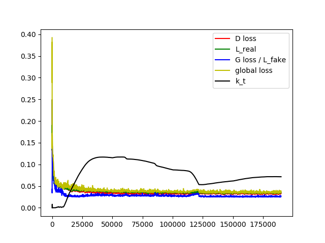
BEGAN: gamma=0.75 learning rate of k=0.001

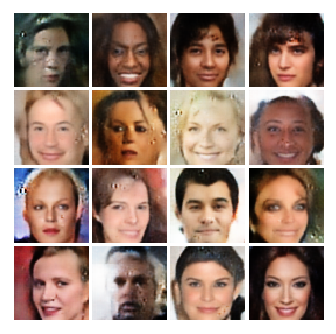
BEGAN: gamma= 0.5 learning rate of k = 0.002

VAE

References

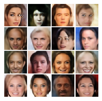
http://wiseodd.github.io/techblog/2016/12/10/variational-autoencoder/ (a good blog to introduce VAE)
https://github.com/wiseodd/generative-models/tree/master/GAN
https://github.com/artcg/BEGAN

Others

Tensorflow style: https://www.tensorflow.org/community/style_guide

A good website to convert latex equation to img(then insert into README): http://www.sciweavers.org/free-online-latex-equation-editor