Release 0.19.1

Bug fixes

• Fixes several bugs when using parametric operations with the default.qubit.torch device on GPU. The device takes the torch_device argument once again to allow running non-parametric QNodes on the GPU. (#1927)

• Fixes a bug where using JAX's jit function on certain QNodes that contain the qml.QubitStateVector operation raised an error with earlier JAX versions (e.g., jax==0.2.10 and jaxlib==0.1.64). (#1924)

Contributors

This release contains contributions from (in alphabetical order):

Josh Izaac, Christina Lee, Romain Moyard, Lee James O'Riordan, Antal Száva.

Release 0.19.0

New features since last release

Differentiable Hartree-Fock solver

• A differentiable Hartree-Fock (HF) solver has been added. It can be used to construct molecular Hamiltonians that can be differentiated with respect to nuclear coordinates and basis-set parameters. (#1610)

  The HF solver computes the integrals over basis functions, constructs the relevant matrices, and performs self-consistent-field iterations to obtain a set of optimized molecular orbital coefficients. These coefficients and the computed integrals over basis functions are used to construct the one- and two-body electron integrals in the molecular orbital basis which can be used to generate a differentiable second-quantized Hamiltonian in the fermionic and qubit basis.

  The following code shows the construction of the Hamiltonian for the hydrogen molecule where the geometry of the molecule is differentiable.

  symbols = ["H", "H"]
  geometry = np.array([[0.0000000000, 0.0000000000, -0.6943528941],
                       [0.0000000000, 0.0000000000,  0.6943528941]], requires_grad=True)
  
  mol = qml.hf.Molecule(symbols, geometry)
  args_mol = [geometry]
  
  hamiltonian = qml.hf.generate_hamiltonian(mol)(*args_mol)

  >>> hamiltonian.coeffs
  tensor([-0.09041082+0.j,  0.17220382+0.j,  0.17220382+0.j,
           0.16893367+0.j,  0.04523101+0.j, -0.04523101+0.j,
          -0.04523101+0.j,  0.04523101+0.j, -0.22581352+0.j,
           0.12092003+0.j, -0.22581352+0.j,  0.16615103+0.j,
           0.16615103+0.j,  0.12092003+0.j,  0.17464937+0.j], requires_grad=True)

  The generated Hamiltonian can be used in a circuit where the atomic coordinates and circuit parameters are optimized simultaneously.

  symbols = ["H", "H"]
  geometry = np.array([[0.0000000000, 0.0000000000, 0.0],
                       [0.0000000000, 0.0000000000, 2.0]], requires_grad=True)
  
  mol = qml.hf.Molecule(symbols, geometry)
  
  dev = qml.device("default.qubit", wires=4)
  params = [np.array([0.0], requires_grad=True)]
  
  def generate_circuit(mol):
      @qml.qnode(dev)
      def circuit(*args):
          qml.BasisState(np.array([1, 1, 0, 0]), wires=[0, 1, 2, 3])
          qml.DoubleExcitation(*args[0][0], wires=[0, 1, 2, 3])
          return qml.expval(qml.hf.generate_hamiltonian(mol)(*args[1:]))
      return circuit
  
  for n in range(25):
  
      mol = qml.hf.Molecule(symbols, geometry)
      args = [params, geometry] # initial values of the differentiable parameters
  
      g_params = qml.grad(generate_circuit(mol), argnum = 0)(*args)
      params = params - 0.5 * g_params[0]
  
      forces = qml.grad(generate_circuit(mol), argnum = 1)(*args)
      geometry = geometry - 0.5 * forces
  
      print(f'Step: {n}, Energy: {generate_circuit(mol)(*args)}, Maximum Force: {forces.max()}')

  In addition, the new Hartree-Fock solver can further be used to optimize the basis set parameters. For details, please refer to the differentiable Hartree-Fock solver documentation.

Integration with Mitiq

• Error mitigation using the zero-noise extrapolation method is now available through the transforms.mitigate_with_zne transform. This transform can integrate with the Mitiq package for unitary folding and extrapolation functionality. (#1813)

  Consider the following noisy device:

  noise_strength = 0.05
  dev = qml.device("default.mixed", wires=2)
  dev = qml.transforms.insert(qml.AmplitudeDamping, noise_strength)(dev)

  We can mitigate the effects of this noise for circuits run on this device by using the added
  transform:

  from mitiq.zne.scaling import fold_global
  from mitiq.zne.inference import RichardsonFactory
  
  n_wires = 2
  n_layers = 2
  
  shapes = qml.SimplifiedTwoDesign.shape(n_wires, n_layers)
  np.random.seed(0)
  w1, w2 = [np.random.random(s) for s in shapes]
  
  @qml.transforms.mitigate_with_zne([1, 2, 3], fold_global, RichardsonFactory.extrapolate)
  @qml.beta.qnode(dev)
  def circuit(w1, w2):
      qml.SimplifiedTwoDesign(w1, w2, wires=range(2))
      return qml.expval(qml.PauliZ(0))

  Now, when we execute circuit, errors will be automatically mitigated:

  >>> circuit(w1, w2)
  0.19113067083636542

Powerful new transforms

• The unitary matrix corresponding to a quantum circuit can now be generated using the new get_unitary_matrix() transform. (#1609) (#1786)

  This transform is fully differentiable across all supported PennyLane autodiff frameworks.

  def circuit(theta):
      qml.RX(theta, wires=1)
      qml.PauliZ(wires=0)
      qml.CNOT(wires=[0, 1])

  >>> theta = torch.tensor(0.3, requires_grad=True)
  >>> matrix = qml.transforms.get_unitary_matrix(circuit)(theta)
  >>> print(matrix)
  tensor([[ 0.9888+0.0000j,  0.0000+0.0000j,  0.0000-0.1494j,  0.0000+0.0000j],
        [ 0.0000+0.0000j,  0.0000+0.1494j,  0.0000+0.0000j, -0.9888+0.0000j],
        [ 0.0000-0.1494j,  0.0000+0.0000j,  0.9888+0.0000j,  0.0000+0.0000j],
        [ 0.0000+0.0000j, -0.9888+0.0000j,  0.0000+0.0000j,  0.0000+0.1494j]],
       grad_fn=<MmBackward>)
  >>> loss = torch.real(torch.trace(matrix))
  >>> loss.backward()
  >>> theta.grad
  tensor(-0.1494)

• Arbitrary two-qubit unitaries can now be decomposed into elementary gates. This functionality has been incorporated into the qml.transforms.unitary_to_rot transform, and is available separately as qml.transforms.two_qubit_decomposition. (#1552)

  As an example, consider the following randomly-generated matrix and circuit that uses it:

  U = np.array([
      [-0.03053706-0.03662692j,  0.01313778+0.38162226j, 0.4101526 -0.81893687j, -0.03864617+0.10743148j],
      [-0.17171136-0.24851809j,  0.06046239+0.1929145j, -0.04813084-0.01748555j, -0.29544883-0.88202604j],
      [ 0.39634931-0.78959795j, -0.25521689-0.17045233j, -0.1391033 -0.09670952j, -0.25043606+0.18393466j],
      [ 0.29599198-0.19573188j,  0.55605806+0.64025769j, 0.06140516+0.35499559j,  0.02674726+0.1563311j ]
  ])
  
  dev = qml.device('default.qubit', wires=2)
  
  @qml.qnode(dev)
  @qml.transforms.unitary_to_rot
  def circuit(x, y):
      qml.QubitUnitary(U, wires=[0, 1])
      return qml.expval(qml.PauliZ(wires=0))

  If we run the circuit, we can see the new decomposition:

  >>> circuit(0.3, 0.4)
  tensor(-0.81295986, requires_grad=True)
  >>> print(qml.draw(circuit)(0.3, 0.4))
  0: ──Rot(2.78, 0.242, -2.28)──╭X──RZ(0.176)───╭C─────────────╭X──Rot(-3.87, 0.321, -2.09)──┤ ⟨Z⟩
  1: ──Rot(4.64, 2.69, -1.56)───╰C──RY(-0.883)──╰X──RY(-1.47)──╰C──Rot(1.68, 0.337, 0.587)───┤

• A new transform, @qml.batch_params, has been added, that makes QNodes handle a batch dimension in trainable parameters. (#1710) (#1761)

  This transform will create multiple circuits, one per batch dimension. As a result, it is both simulator and hardware compatible.

  @qml.batch_params
  @qml.beta.qnode(dev)
  def circuit(x, weights):
      qml.RX(x, wires=0)
      qml.RY(0.2, wires=1)
      qml.templates.StronglyEntanglingLayers(weights, wires=[0, 1, 2])
      return qml.expval(qml.Hadamard(0))

  The qml.batch_params decorator allows us to pass arguments x and weights that have a batch dimension. For example,

  >>> batch_size = 3
  >>> x = np.linspace(0.1, 0.5, batch_size)
  >>> weights = np.random.random((batch_size, 10, 3, 3))

  If we evaluate the QNode with these inputs, we will get an output of shape (batch_size,):

  >>> circuit(x, weights)
  tensor([0.08569816, 0.12619101, 0.21122004], requires_grad=True)

• The insert transform has now been added, providing a way to insert single-qubit operations into a quantum circuit. The transform can apply to quantum functions, tapes, and devices. (#1795)

  The following QNode can be transformed to add noise to the circuit:

  dev = qml.device("default.mixed", wires=2)
  
  @qml.qnode(dev)
  @qml.transforms.insert(qml.AmplitudeDamping, 0.2, position="end")
  def f(w, x, y, z):
      qml.RX(w, wires=0)
      qml.RY(x, wires=1)
      qml.CNOT(wires=[0, 1])
      qml.RY(y, wires=0)
      qml.RX(z, wires=1)
      return qml.expval(qml.PauliZ(0) @ qml.PauliZ(1))

  Executions of this circuit will differ from the noise-free value:

  >>> f(0.9, 0.4, 0.5, 0.6)
  tensor(0.754847, requires_grad=True)
  >>> print(qml.draw(f)(0.9, 0.4, 0.5, 0.6))
   0: ──RX(0.9)──╭C──RY(0.5)──AmplitudeDamping(0.2)──╭┤ ⟨Z ⊗ Z⟩
   1: ──RY(0.4)──╰X──RX(0.6)──AmplitudeDamping(0.2)──╰┤ ⟨Z ⊗ Z⟩

• Common tape expansion functions are now available in qml.transforms, alongside a new create_expand_fn function for easily creating expansion functions from stopping criteria. (#1734) (#1760)

  create_expand_fn takes the default depth to which the expansion function should expand a tape, a stopping criterion, an optional device, and a docstring to be set for the created function. The stopping criterion must take a q...

Release 0.18.0-post2

A minor post-release to update the PennyLane documentation navigation bar.

Release 0.18.0-post1

A minor post-release to update the PennyLane documentation navigation bar to include a link to the demonstrations.

Release 0.18.0

New features since last release

PennyLane now comes packaged with lightning.qubit

• The C++-based lightning.qubit device is now included with installations of PennyLane. (#1663)

  The lightning.qubit device is a fast state-vector simulator equipped with the efficient adjoint method for differentiating quantum circuits, check out the plugin release notes for more details! The device can be accessed in the following way:

  import pennylane as qml
  
  wires = 3
  layers = 2
  dev = qml.device("lightning.qubit", wires=wires)
  
  @qml.qnode(dev, diff_method="adjoint")
  def circuit(weights):
      qml.templates.StronglyEntanglingLayers(weights, wires=range(wires))
      return qml.expval(qml.PauliZ(0))
  
  weights = qml.init.strong_ent_layers_normal(layers, wires, seed=1967)

  Evaluating circuits and their gradients on the device can be achieved using the standard approach:

  >>> print(f"Circuit evaluated: {circuit(weights)}")
  Circuit evaluated: 0.9801286266677633
  >>> print(f"Circuit gradient:\n{qml.grad(circuit)(weights)}")
  Circuit gradient:
  [[[-9.35301749e-17 -1.63051504e-01 -4.14810501e-04]
    [-7.88816484e-17 -1.50136528e-04 -1.77922957e-04]
    [-5.20670796e-17 -3.92874550e-02  8.14523075e-05]]
  
   [[-1.14472273e-04  3.85963953e-02 -9.39190132e-18]
    [-5.76791765e-05 -9.78478343e-02  0.00000000e+00]
    [ 0.00000000e+00  0.00000000e+00  0.00000000e+00]]]

  The adjoint method operates after a forward pass by iteratively applying inverse gates to scan backwards through the circuit. The method is already available in PennyLane's default.qubit device, but the version provided by lightning.qubit integrates with the C++ backend and is more performant, as shown in the plot below: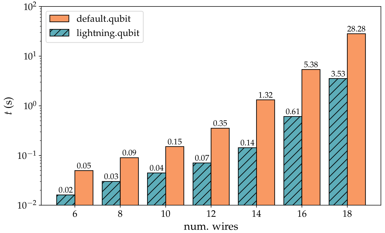

  

Support for native backpropagation using PyTorch

• The built-in PennyLane simulator default.qubit now supports backpropogation with PyTorch. (#1360) (#1598)

  As a result, default.qubit can now use end-to-end classical backpropagation as a means to compute gradients. End-to-end backpropagation can be faster than the parameter-shift rule for computing quantum gradients when the number of parameters to be optimized is large. This is now the default differentiation method when using default.qubit with PyTorch.

  Using this method, the created QNode is a 'white-box' that is tightly integrated with your PyTorch computation, including TorchScript and GPU support.

  x = torch.tensor(0.43316321, dtype=torch.float64, requires_grad=True)
  y = torch.tensor(0.2162158, dtype=torch.float64, requires_grad=True)
  z = torch.tensor(0.75110998, dtype=torch.float64, requires_grad=True)
  
  p = torch.tensor([x, y, z], requires_grad=True)
  dev = qml.device("default.qubit", wires=1)
  
  @qml.qnode(dev, interface="torch", diff_method="backprop")
  def circuit(x):
      qml.Rot(x[0], x[1], x[2], wires=0)
      return qml.expval(qml.PauliZ(0))
  
  res = circuit(p)
  res.backward()

  >>> res = circuit(p)
  >>> res.backward()
  >>> print(p.grad)
  tensor([-9.1798e-17, -2.1454e-01, -1.0511e-16], dtype=torch.float64)

Improved quantum optimization methods

• The RotosolveOptimizer now can tackle general parametrized circuits, and is no longer restricted to single-qubit Pauli rotations. (#1489)

  This includes:

  • layers of gates controlled by the same parameter,
  • controlled variants of parametrized gates, and
  • Hamiltonian time evolution.

  Note that the eigenvalue spectrum of the gate generator needs to be known to use RotosolveOptimizer for a general gate, and it is required to produce equidistant frequencies. For details see Vidal and Theis, 2018 and Wierichs, Izaac, Wang, Lin 2021.

  Consider a circuit with a mixture of Pauli rotation gates, controlled Pauli rotations, and single-parameter layers of Pauli rotations:

  dev = qml.device('default.qubit', wires=3, shots=None)
  
  @qml.qnode(dev)
  def cost_function(rot_param, layer_par, crot_param):
      for i, par in enumerate(rot_param):
          qml.RX(par, wires=i)
      for w in dev.wires:
          qml.RX(layer_par, wires=w)
      for i, par in enumerate(crot_param):
          qml.CRY(par, wires=[i, (i+1) % 3])
  
      return qml.expval(qml.PauliZ(0) @ qml.PauliZ(1) @ qml.PauliZ(2))

  This cost function has one frequency for each of the first RX rotation angles, three frequencies for the layer of RX gates that depend on layer_par, and two frequencies for each of the CRY gate parameters. Rotosolve can then be used to minimize the cost_function:

  # Initial parameters
  init_param = [
      np.array([0.3, 0.2, 0.67], requires_grad=True),
      np.array(1.1, requires_grad=True),
      np.array([-0.2, 0.1, -2.5], requires_grad=True),
  ]
  # Numbers of frequencies per parameter
  num_freqs = [[1, 1, 1], 3, [2, 2, 2]]
  
  opt = qml.RotosolveOptimizer()
  param = init_param.copy()

  In addition, the optimization technique for the Rotosolve substeps can be chosen via the optimizer and optimizer_kwargs keyword arguments and the minimized cost of the intermediate univariate reconstructions can be read out via full_output, including the cost after the full Rotosolve step:

  for step in range(3):
      param, cost, sub_cost = opt.step_and_cost(
          cost_function,
          *param,
          num_freqs=num_freqs,
          full_output=True,
          optimizer="brute",
      )
      print(f"Cost before step: {cost}")
      print(f"Minimization substeps: {np.round(sub_cost, 6)}")

  Cost before step: 0.042008210392535605
  Minimization substeps: [-0.230905 -0.863336 -0.980072 -0.980072 -1.       -1.       -1.      ]
  Cost before step: -0.999999999068121
  Minimization substeps: [-1. -1. -1. -1. -1. -1. -1.]
  Cost before step: -1.0
  Minimization substeps: [-1. -1. -1. -1. -1. -1. -1.]

  For usage details please consider the docstring of the optimizer.

Faster, trainable, Hamiltonian simulations

• Hamiltonians are now trainable with respect to their coefficients. (#1483)

  from pennylane import numpy as np
  
  dev = qml.device("default.qubit", wires=2)
  @qml.qnode(dev)
  def circuit(coeffs, param):
      qml.RX(param, wires=0)
      qml.RY(param, wires=0)
      return qml.expval(
          qml.Hamiltonian(coeffs, [qml.PauliX(0), qml.PauliZ(0)], simplify=True)
      )
  
  coeffs = np.array([-0.05, 0.17])
  param = np.array(1.7)
  grad_fn = qml.grad(circuit)

  >>> grad_fn(coeffs, param)
  (array([-0.12777055,  0.0166009 ]), array(0.0917819))

  Furthermore, a gradient recipe for Hamiltonian coefficients has been added. This makes it possible to compute parameter-shift gradients of these coefficients on devices that natively support Hamiltonians. (#1551)

• Hamiltonians are now natively supported on the default.qubit device if shots=None. This makes VQE workflows a lot faster in some cases. (#1551) (#1596)

  

• The Hamiltonian can now store grouping information, which can be accessed by a device to speed up computations of the expectation value of a Hamiltonian. (#1515)

  obs = [qml.PauliX(0), qml.PauliX(1), qml.PauliZ(0)]
  coeffs = np.array([1., 2., 3.])
  H = qml.Hamiltonian(coeffs, obs, grouping_type='qwc')

  Initialization with a grouping_type other than None stores the indices
  required to make groups of commuting observables and their coefficients.

  >>> H.grouping_indices
  [[0, 1], [2]]

Create multi-circuit quantum transforms and custom gradient rules

• Custom gradient transforms can now be created using the new @qml.gradients.gradient_transform decorator on a batch-tape transform. (#1589)

  Quantum gradient transforms are a specific case of qml.batch_transform.

  Supported gradient transforms must be of the following form:

  @qml.gradients.gradient_transform
  def my_custom_gradient(tape, argnum=None, **kwargs):
      ...
      return gradient_tapes, processing_fn

  Various built-in quantum gradient transforms are provided within the qml.gradients module, including qml.gradients.param_shift. Once defined, quantum gradient transforms can be applied directly to QNodes:

  >>> @qml.qnode(dev)
  ... def circuit(x):
  ...     qml.RX(x, wires=0)
  ...     qml.CNOT(wires=[0, 1])
  ...     return qml.expval(qml.PauliZ(0))
  >>> circuit(0.3)
  tensor(0.95533649, requires_grad=True)
  >>> qml.gradients.param_shift(circui...

Release 0.17.0

New features since the last release

Circuit optimization

• PennyLane can now perform quantum circuit optimization using the top-level transform qml.compile. The compile transform allows you to chain together sequences of tape and quantum function transforms into custom circuit optimization pipelines. (#1475)

  For example, take the following decorated quantum function:

  dev = qml.device('default.qubit', wires=[0, 1, 2])
  
  @qml.qnode(dev)
  @qml.compile()
  def qfunc(x, y, z):
      qml.Hadamard(wires=0)
      qml.Hadamard(wires=1)
      qml.Hadamard(wires=2)
      qml.RZ(z, wires=2)
      qml.CNOT(wires=[2, 1])
      qml.RX(z, wires=0)
      qml.CNOT(wires=[1, 0])
      qml.RX(x, wires=0)
      qml.CNOT(wires=[1, 0])
      qml.RZ(-z, wires=2)
      qml.RX(y, wires=2)
      qml.PauliY(wires=2)
      qml.CZ(wires=[1, 2])
      return qml.expval(qml.PauliZ(wires=0))

  The default behaviour of qml.compile is to apply a sequence of three transforms: commute_controlled, cancel_inverses, and then merge_rotations.

  >>> print(qml.draw(qfunc)(0.2, 0.3, 0.4))
   0: ──H───RX(0.6)──────────────────┤ ⟨Z⟩
   1: ──H──╭X────────────────────╭C──┤
   2: ──H──╰C────────RX(0.3)──Y──╰Z──┤

  The qml.compile transform is flexible and accepts a custom pipeline of tape and quantum function transforms (you can even write your own!). For example, if we wanted to only push single-qubit gates through controlled gates and cancel adjacent inverses, we could do:

  from pennylane.transforms import commute_controlled, cancel_inverses
  pipeline = [commute_controlled, cancel_inverses]
  
  @qml.qnode(dev)
  @qml.compile(pipeline=pipeline)
  def qfunc(x, y, z):
      qml.Hadamard(wires=0)
      qml.Hadamard(wires=1)
      qml.Hadamard(wires=2)
      qml.RZ(z, wires=2)
      qml.CNOT(wires=[2, 1])
      qml.RX(z, wires=0)
      qml.CNOT(wires=[1, 0])
      qml.RX(x, wires=0)
      qml.CNOT(wires=[1, 0])
      qml.RZ(-z, wires=2)
      qml.RX(y, wires=2)
      qml.PauliY(wires=2)
      qml.CZ(wires=[1, 2])
      return qml.expval(qml.PauliZ(wires=0))

  >>> print(qml.draw(qfunc)(0.2, 0.3, 0.4))
   0: ──H───RX(0.4)──RX(0.2)────────────────────────────┤ ⟨Z⟩
   1: ──H──╭X───────────────────────────────────────╭C──┤
   2: ──H──╰C────────RZ(0.4)──RZ(-0.4)──RX(0.3)──Y──╰Z──┤

  The following compilation transforms have been added and are also available to use, either independently, or within a qml.compile pipeline:

  • commute_controlled: push commuting single-qubit gates through controlled operations. (#1464)

  • cancel_inverses: removes adjacent pairs of operations that cancel out. (#1455)

  • merge_rotations: combines adjacent rotation gates of the same type into a single gate, including controlled rotations. (#1455)

  • single_qubit_fusion: acts on all sequences of single-qubit operations in a quantum function, and converts each sequence to a single Rot gate. (#1458)

  For more details on qml.compile and the available compilation transforms, see the compilation documentation.

QNodes are even more powerful

• Computational basis samples directly from the underlying device can now be returned directly from QNodes via qml.sample(). (#1441)

dev = qml.device("default.qubit", wires=3, shots=5)

@qml.qnode(dev)
def circuit_1():
    qml.Hadamard(wires=0)
    qml.Hadamard(wires=1)
    return qml.sample()

@qml.qnode(dev)
def circuit_2():
    qml.Hadamard(wires=0)
    qml.Hadamard(wires=1)
    return qml.sample(wires=[0,2])    # no observable provided and wires specified

>>> print(circuit_1())
[[1, 0, 0],
 [1, 1, 0],
 [1, 0, 0],
 [0, 0, 0],
 [0, 1, 0]]

>>> print(circuit_2())
[[1, 0],
 [1, 0],
 [1, 0],
 [0, 0],
 [0, 0]]

>>> print(qml.draw(circuit_2)())
 0: ──H──╭┤ Sample[basis]
 1: ──H──│┤
 2: ─────╰┤ Sample[basis]

• The new qml.apply function can be used to add operations that might have already been instantiated elsewhere to the QNode and other queuing contexts: (#1433)

  op = qml.RX(0.4, wires=0)
  dev = qml.device("default.qubit", wires=2)
  
  @qml.qnode(dev)
  def circuit(x):
      qml.RY(x, wires=0)
      qml.apply(op)
      return qml.expval(qml.PauliZ(0))

  >>> print(qml.draw(circuit)(0.6))
  0: ──RY(0.6)──RX(0.4)──┤ ⟨Z⟩

  Previously instantiated measurements can also be applied to QNodes.

Device Resource Tracker

• The new Device Tracker capabilities allows for flexible and versatile tracking of executions, even inside parameter-shift gradients. This functionality will improve the ease of monitoring large batches and remote jobs. (#1355)

  dev = qml.device('default.qubit', wires=1, shots=100)
  
  @qml.qnode(dev, diff_method="parameter-shift")
  def circuit(x):
      qml.RX(x, wires=0)
      return qml.expval(qml.PauliZ(0))
  
  x = np.array(0.1)
  
  with qml.Tracker(circuit.device) as tracker:
      qml.grad(circuit)(x)

  >>> tracker.totals
  {'executions': 3, 'shots': 300, 'batches': 1, 'batch_len': 2}
  >>> tracker.history
  {'executions': [1, 1, 1],
   'shots': [100, 100, 100],
   'batches': [1],
   'batch_len': [2]}
  >>> tracker.latest
  {'batches': 1, 'batch_len': 2}

  Users can also provide a custom function to the callback keyword that gets called each time the information is updated. This functionality allows users to monitor remote jobs or large parameter-shift batches.

  >>> def shots_info(totals, history, latest):
  ...     print("Total shots: ", totals['shots'])
  >>> with qml.Tracker(circuit.device, callback=shots_info) as tracker:
  ...     qml.grad(circuit)(0.1)
  Total shots:  100
  Total shots:  200
  Total shots:  300
  Total shots:  300

Containerization support

• Docker support for building PennyLane with support for all interfaces (TensorFlow, Torch, and Jax), as well as device plugins and QChem, for GPUs and CPUs, has been added. (#1391)

  The build process using Docker and make requires that the repository source code is cloned or downloaded from GitHub. Visit the the detailed description for an extended list of options.

Improved Hamiltonian simulations

• Added a sparse Hamiltonian observable and the functionality to support computing its expectation value with default.qubit. (#1398)

  For example, the following QNode returns the expectation value of a sparse Hamiltonian:

  dev = qml.device("default.qubit", wires=2)
  
  @qml.qnode(dev, diff_method="parameter-shift")
  def circuit(param, H):
      qml.PauliX(0)
      qml.SingleExcitation(param, wires=[0, 1])
      return qml.expval(qml.SparseHamiltonian(H, [0, 1]))

  We can execute this QNode, passing in a sparse identity matrix:

  >>> print(circuit([0.5], scipy.sparse.eye(4).tocoo()))
  0.9999999999999999

  The expectation value of the sparse Hamiltonian is computed directly, which leads to executions that are faster by orders of magnitude. Note that "parameter-shift" is the only differentiation method that is currently supported when the observable is a sparse Hamiltonian.

• VQE problems can now be intuitively set up by passing the Hamiltonian as an observable. (#1474)

  dev = qml.device("default.qubit", wires=2)
  H = qml.Hamiltonian([1., 2., 3.],  [qml.PauliZ(0), qml.PauliY(0), qml.PauliZ(1)])
  w = qml.init.strong_ent_layers_uniform(1, 2, seed=1967)
  
  @qml.qnode(dev)
  def circuit(w):
      qml.templates.StronglyEntanglingLayers(w, wires=range(2))
      return qml.expval(H)

  >>> print(circuit(w))
  -1.5133943637878295
  >>> print(qml.grad(circuit)(w))
  [[[-8.32667268e-17  1.39122955e+00 -9.12462052e-02]
  [ 1.02348685e-16 -7.77143238e-01 -1.74708049e-01]]]

  Note that other measurement types like var(H) or sample(H), as well as multiple expectations like expval(H1), expval(H2) are not supported.

• Added functionality to compute the sparse matrix representation of a qml.Hamiltonian object. (#1394)

New gradients module

• A new gradients module qml.gradients has been added, which provides differentiable quantum gradient transforms. (#1476) (#1479) (#1486)

  Available quantum gradient transforms include:

  • qml.gradients.finite_diff
  • qml.gradients.param_shift
  • qml.gradients.param_shift_cv

  For example,

  >>> params = np.array([0.3,0.4,0.5], requires_grad=True)
  >>> with qml.tape.JacobianTape() as tape:
  ...     qml.RX(params[0], wires=0)
  ...     qml.RY(params[1], wires=0)
  ...     qml.RX(params[2], wires=0)
  ...   ...

Release 0.16.0

New features since last release

First class support for quantum kernels

• The new qml.kernels module provides basic functionalities for working with quantum kernels as well as post-processing methods to mitigate sampling errors and device noise: (#1102)

  num_wires = 6
  wires = range(num_wires)
  dev = qml.device('default.qubit', wires=wires)
  
  @qml.qnode(dev)
  def kernel_circuit(x1, x2):
      qml.templates.AngleEmbedding(x1, wires=wires)
      qml.adjoint(qml.templates.AngleEmbedding)(x2, wires=wires)
      return qml.probs(wires)
  
  kernel = lambda x1, x2: kernel_circuit(x1, x2)[0]
  X_train = np.random.random((10, 6))
  X_test = np.random.random((5, 6))
  
  # Create symmetric square kernel matrix (for training)
  K = qml.kernels.square_kernel_matrix(X_train, kernel)
  
  # Compute kernel between test and training data.
  K_test = qml.kernels.kernel_matrix(X_train, X_test, kernel)
  K1 = qml.kernels.mitigate_depolarizing_noise(K, num_wires, method='single')

Extract the fourier representation of quantum circuits

• PennyLane now has a fourier module, which hosts a growing library of methods that help with investigating the Fourier representation of functions implemented by quantum circuits. The Fourier representation can be used to examine and characterize the expressivity of the quantum circuit. (#1160) (#1378)

  For example, one can plot distributions over Fourier series coefficients like this one:

  

Seamless support for working with the Pauli group

• Added functionality for constructing and manipulating the Pauli group (#1181).

  The function qml.grouping.pauli_group provides a generator to easily loop over the group, or construct and store it in its entirety. For example, we can construct the single-qubit Pauli group like so:

  >>> from pennylane.grouping import pauli_group
  >>> pauli_group_1_qubit = list(pauli_group(1))
  >>> pauli_group_1_qubit
  [Identity(wires=[0]), PauliZ(wires=[0]), PauliX(wires=[0]), PauliY(wires=[0])]

  We can multiply together its members at the level of Pauli words using the pauli_mult and pauli_multi_with_phase functions. This can be done on arbitrarily-labeled wires as well, by defining a wire map.

  >>> from pennylane.grouping import pauli_group, pauli_mult
  >>> wire_map = {'a' : 0, 'b' : 1, 'c' : 2}
  >>> pg = list(pauli_group(3, wire_map=wire_map))
  >>> pg[3]
  PauliZ(wires=['b']) @ PauliZ(wires=['c'])
  >>> pg[55]
  PauliY(wires=['a']) @ PauliY(wires=['b']) @ PauliZ(wires=['c'])
  >>> pauli_mult(pg[3], pg[55], wire_map=wire_map)
  PauliY(wires=['a']) @ PauliX(wires=['b'])

  Functions for conversion of Pauli observables to strings (and back) are included.

  >>> from pennylane.grouping import pauli_word_to_string, string_to_pauli_word
  >>> pauli_word_to_string(pg[55], wire_map=wire_map)
  'YYZ'
  >>> string_to_pauli_word('ZXY', wire_map=wire_map)
  PauliZ(wires=['a']) @ PauliX(wires=['b']) @ PauliY(wires=['c'])

  Calculation of the matrix representation for arbitrary Paulis and wire maps is now also supported.

  >>> from pennylane.grouping import pauli_word_to_matrix
  >>> wire_map = {'a' : 0, 'b' : 1}
  >>> pauli_word = qml.PauliZ('b')  # corresponds to Pauli 'IZ'
  >>> pauli_word_to_matrix(pauli_word, wire_map=wire_map)
  array([[ 1.,  0.,  0.,  0.],
         [ 0., -1.,  0., -0.],
         [ 0.,  0.,  1.,  0.],
         [ 0., -0.,  0., -1.]])

New transforms

• The qml.specs QNode transform creates a function that returns specifications or details about the QNode, including depth, number of gates, and number of gradient executions required. (#1245)

  For example:

  dev = qml.device('default.qubit', wires=4)
  
  @qml.qnode(dev, diff_method='parameter-shift')
  def circuit(x, y):
      qml.RX(x[0], wires=0)
      qml.Toffoli(wires=(0, 1, 2))
      qml.CRY(x[1], wires=(0, 1))
      qml.Rot(x[2], x[3], y, wires=0)
      return qml.expval(qml.PauliZ(0)), qml.expval(qml.PauliX(1))

  We can now use the qml.specs transform to generate a function that returns details and resource information:

  >>> x = np.array([0.05, 0.1, 0.2, 0.3], requires_grad=True)
  >>> y = np.array(0.4, requires_grad=False)
  >>> specs_func = qml.specs(circuit)
  >>> specs_func(x, y)
  {'gate_sizes': defaultdict(int, {1: 2, 3: 1, 2: 1}),
   'gate_types': defaultdict(int, {'RX': 1, 'Toffoli': 1, 'CRY': 1, 'Rot': 1}),
   'num_operations': 4,
   'num_observables': 2,
   'num_diagonalizing_gates': 1,
   'num_used_wires': 3,
   'depth': 4,
   'num_trainable_params': 4,
   'num_parameter_shift_executions': 11,
   'num_device_wires': 4,
   'device_name': 'default.qubit',
   'diff_method': 'parameter-shift'}

  The tape methods get_resources and get_depth are superseded by specs and will be deprecated after one release cycle.

• Adds a decorator @qml.qfunc_transform to easily create a transformation that modifies the behaviour of a quantum function.
  (#1315)

  For example, consider the following transform, which scales the parameter of all RX gates by :math:x \rightarrow \sin(a) \sqrt{x}, and the parameters of all RY gates by :math:y \rightarrow \cos(a * b) y:

  @qml.qfunc_transform
  def my_transform(tape, a, b):
      for op in tape.operations + tape.measurements:
          if op.name == "RX":
              x = op.parameters[0]
              qml.RX(qml.math.sin(a) * qml.math.sqrt(x), wires=op.wires)
          elif op.name == "RY":
              y = op.parameters[0]
              qml.RX(qml.math.cos(a * b) * y, wires=op.wires)
          else:
              op.queue()

  We can now apply this transform to any quantum function:

  dev = qml.device("default.qubit", wires=2)
  
  def ansatz(x):
      qml.Hadamard(wires=0)
      qml.RX(x[0], wires=0)
      qml.RY(x[1], wires=1)
      qml.CNOT(wires=[0, 1])
  
  @qml.qnode(dev)
  def circuit(params, transform_weights):
      qml.RX(0.1, wires=0)
  
      # apply the transform to the ansatz
      my_transform(*transform_weights)(ansatz)(params)
  
      return qml.expval(qml.PauliZ(1))

  We can print this QNode to show that the qfunc transform is taking place:

  >>> x = np.array([0.5, 0.3], requires_grad=True)
  >>> transform_weights = np.array([0.1, 0.6], requires_grad=True)
  >>> print(qml.draw(circuit)(x, transform_weights))
   0: ──RX(0.1)────H──RX(0.0706)──╭C──┤
   1: ──RX(0.299)─────────────────╰X──┤ ⟨Z⟩

  Evaluating the QNode, as well as the derivative, with respect to the gate parameter and the transform weights:

  >>> circuit(x, transform_weights)
  tensor(0.00672829, requires_grad=True)
  >>> qml.grad(circuit)(x, transform_weights)
  (array([ 0.00671711, -0.00207359]), array([6.69695008e-02, 3.73694364e-06]))

• Adds a hamiltonian_expand tape transform. This takes a tape ending in qml.expval(H), where H is a Hamiltonian, and maps it to a collection of tapes which can be executed and passed into a post-processing function yielding the expectation value. (#1142)

  Example use:

  H = qml.PauliZ(0) + 3 * qml.PauliZ(0) @ qml.PauliX(1)
  
  with qml.tape.QuantumTape() as tape:
      qml.Hadamard(wires=1)
      qml.expval(H)
  
  tapes, fn = qml.transforms.hamiltonian_expand(tape)

  We can now evaluate the transformed tapes, and apply the post-processing function:

  >>> dev = qml.device("default.qubit", wires=3)
  >>> res = dev.batch_execute(tapes)
  >>> fn(res)
  3.999999999999999

• The quantum_monte_carlo transform has been added, allowing an input circuit to be transformed into the full quantum Monte Carlo algorithm. (#1316)

  Suppose we want to measure the expectation value of the sine squared function according to a standard normal distribution. We can calculate the expectation value analytically as 0.432332, but we can also estimate using the quantum Monte Carlo algorithm. The first step is to discretize the problem:

  from scipy.stats import norm
  
  m = 5
  M = 2 ** m
  
  xmax = np.pi  # bound to region [-pi, pi]
  xs = np.linspace(-xmax, xmax, M)
  
  probs = np.array([norm().pdf(x) for x in xs])
  probs /= np.sum(probs)
  
  func = lambda i: np.sin(xs[i]) ** 2
  r_rotations = np.array([2 * np.arcsin(np.sqrt(func(i))) for i in range(M)])

  The quantum_monte_carlo transform can then be used:

  from pennylane.templates.state_preparations.mottonen import (
      _uniform_rotation_dagger as r_unitary,
  )
  
  n = 6
  N = 2 ** n
  
  a_wires = range(m)
  wires = range(m + 1)
  target_wire = m
  estimation_wires = range(m + 1, n + m + 1)
  
  dev = qml.device("default.qubit", wires=(n + m + 1))
  
  def fn():
      qml.templates.MottonenStatePreparation(np.sqrt(probs), wires=a_wires)
      r_unitary(qml.RY, r_rotations, control_wires=a_wires[::-1], target_wire=target_wire)
  
  @qml.qnode(dev)
  def qmc():
      qml.quantum_monte_carlo(fn, wires, target_wire, estimation_wires)()
      return qml.probs(estimation_wires)...

Release 0.15.1

Bug fixes

• Fixes two bugs in the parameter-shift Hessian. (#1260)

  • Fixes a bug where having an unused parameter in the Autograd interface would result in an indexing error during backpropagation.

  • The parameter-shift Hessian only supports the two-term parameter-shift rule currently, so raises an error if asked to differentiate any unsupported gates (such as the controlled rotation gates).

• A bug which resulted in qml.adjoint() and qml.inv() failing to work with templates has been fixed. (#1243)

• Deprecation warning instances in PennyLane have been changed to UserWarning, to account for recent changes to how Python warnings are filtered in PEP565. (#1211)

• The version requirement for PySCF has been modified to allow for pyscf>=1.7.2. (#1254)

Documentation

• Updated the order of the parameters to the GaussianState operation to match the way that the PennyLane-SF plugin uses them. (#1255)

Contributors

This release contains contributions from (in alphabetical order):

Josh Izaac, Maria Schuld, Antal Száva.

Release 0.15.0

New features since last release

Better and more flexible shot control

• Adds a new optimizer qml.ShotAdaptiveOptimizer, a gradient-descent optimizer where the shot rate is adaptively calculated using the variances of the parameter-shift gradient. (#1139)

  By keeping a running average of the parameter-shift gradient and the variance of the parameter-shift gradient, this optimizer frugally distributes a shot budget across the partial derivatives of each parameter.

  In addition, if computing the expectation value of a Hamiltonian, weighted random sampling can be used to further distribute the shot budget across the local terms from which the Hamiltonian is constructed.

  This optimizer is based on both the iCANS1 and Rosalin shot-adaptive optimizers.

  Once constructed, the cost function can be passed directly to the optimizer's step method. The attribute opt.total_shots_used can be used to track the number of shots per iteration.

  >>> coeffs = [2, 4, -1, 5, 2]
  >>> obs = [
  ...   qml.PauliX(1),
  ...   qml.PauliZ(1),
  ...   qml.PauliX(0) @ qml.PauliX(1),
  ...   qml.PauliY(0) @ qml.PauliY(1),
  ...   qml.PauliZ(0) @ qml.PauliZ(1)
  ... ]
  >>> H = qml.Hamiltonian(coeffs, obs)
  >>> dev = qml.device("default.qubit", wires=2, shots=100)
  >>> cost = qml.ExpvalCost(qml.templates.StronglyEntanglingLayers, H, dev)
  >>> params = qml.init.strong_ent_layers_uniform(n_layers=2, n_wires=2)
  >>> opt = qml.ShotAdaptiveOptimizer(min_shots=10)
  >>> for i in range(5):
  ...    params = opt.step(cost, params)
  ...    print(f"Step {i}: cost = {cost(params):.2f}, shots_used = {opt.total_shots_used}")
  Step 0: cost = -5.68, shots_used = 240
  Step 1: cost = -2.98, shots_used = 336
  Step 2: cost = -4.97, shots_used = 624
  Step 3: cost = -5.53, shots_used = 1054
  Step 4: cost = -6.50, shots_used = 1798

• Batches of shots can now be specified as a list, allowing measurement statistics to be course-grained with a single QNode evaluation. (#1103)

  >>> shots_list = [5, 10, 1000]
  >>> dev = qml.device("default.qubit", wires=2, shots=shots_list)

  When QNodes are executed on this device, a single execution of 1015 shots will be submitted. However, three sets of measurement statistics will be returned; using the first 5 shots, second set of 10 shots, and final 1000 shots, separately.

  For example, executing a circuit with two outputs will lead to a result of shape (3, 2):

  >>> @qml.qnode(dev)
  ... def circuit(x):
  ...     qml.RX(x, wires=0)
  ...     qml.CNOT(wires=[0, 1])
  ...     return qml.expval(qml.PauliZ(0) @ qml.PauliX(1)), qml.expval(qml.PauliZ(0))
  >>> circuit(0.5)
  [[0.33333333 1.        ]
   [0.2        1.        ]
   [0.012      0.868     ]]

  This output remains fully differentiable.

• The number of shots can now be specified on a per-call basis when evaluating a QNode. (#1075).

  For this, the qnode should be called with an additional shots keyword argument:

  >>> dev = qml.device('default.qubit', wires=1, shots=10) # default is 10
  >>> @qml.qnode(dev)
  ... def circuit(a):
  ...     qml.RX(a, wires=0)
  ...     return qml.sample(qml.PauliZ(wires=0))
  >>> circuit(0.8)
  [ 1  1  1 -1 -1  1  1  1  1  1]
  >>> circuit(0.8, shots=3)
  [ 1  1  1]
  >>> circuit(0.8)
  [ 1  1  1 -1 -1  1  1  1  1  1]

New differentiable quantum transforms

A new module is available, qml.transforms, which contains differentiable quantum transforms. These are functions that act on QNodes, quantum functions, devices, and tapes, transforming them while remaining fully differentiable.

• A new adjoint transform has been added. (#1111) (#1135)

  This new method allows users to apply the adjoint of an arbitrary sequence of operations.

  def subroutine(wire):
      qml.RX(0.123, wires=wire)
      qml.RY(0.456, wires=wire)
  
  dev = qml.device('default.qubit', wires=1)
  @qml.qnode(dev)
  def circuit():
      subroutine(0)
      qml.adjoint(subroutine)(0)
      return qml.expval(qml.PauliZ(0))

  This creates the following circuit:

  >>> print(qml.draw(circuit)())
  0: --RX(0.123)--RY(0.456)--RY(-0.456)--RX(-0.123)--| <Z>

  Directly applying to a gate also works as expected.

  qml.adjoint(qml.RX)(0.123, wires=0) # applies RX(-0.123)

• A new transform qml.ctrl is now available that adds control wires to subroutines. (#1157)

  def my_ansatz(params):
     qml.RX(params[0], wires=0)
     qml.RZ(params[1], wires=1)
  
  # Create a new operation that applies `my_ansatz`
  # controlled by the "2" wire.
  my_ansatz2 = qml.ctrl(my_ansatz, control=2)
  
  @qml.qnode(dev)
  def circuit(params):
      my_ansatz2(params)
      return qml.state()

  This is equivalent to:

  @qml.qnode(...)
  def circuit(params):
      qml.CRX(params[0], wires=[2, 0])
      qml.CRZ(params[1], wires=[2, 1])
      return qml.state()

• The qml.transforms.classical_jacobian transform has been added. (#1186)

  This transform returns a function to extract the Jacobian matrix of the classical part of a QNode, allowing the classical dependence between the QNode arguments and the quantum gate arguments to be extracted.

  For example, given the following QNode:

  >>> @qml.qnode(dev)
  ... def circuit(weights):
  ...     qml.RX(weights[0], wires=0)
  ...     qml.RY(weights[0], wires=1)
  ...     qml.RZ(weights[2] ** 2, wires=1)
  ...     return qml.expval(qml.PauliZ(0))

  We can use this transform to extract the relationship :math:f: \mathbb{R}^n \rightarrow\mathbb{R}^m between the input QNode arguments :math:w and the gate arguments :math:g, for a given value of the QNode arguments:

  >>> cjac_fn = qml.transforms.classical_jacobian(circuit)
  >>> weights = np.array([1., 1., 1.], requires_grad=True)
  >>> cjac = cjac_fn(weights)
  >>> print(cjac)
  [[1. 0. 0.]
   [1. 0. 0.]
   [0. 0. 2.]]

  The returned Jacobian has rows corresponding to gate arguments, and columns corresponding to QNode arguments; that is, :math:J_{ij} = \frac{\partial}{\partial g_i} f(w_j).

More operations and templates

• Added the SingleExcitation two-qubit operation, which is useful for quantum chemistry applications. (#1121)

  It can be used to perform an SO(2) rotation in the subspace spanned by the states :math:|01\rangle and :math:|10\rangle. For example, the following circuit performs the transformation :math:|10\rangle \rightarrow \cos(\phi/2)|10\rangle - \sin(\phi/2)|01\rangle:

  dev = qml.device('default.qubit', wires=2)
  
  @qml.qnode(dev)
  def circuit(phi):
      qml.PauliX(wires=0)
      qml.SingleExcitation(phi, wires=[0, 1])

  The SingleExcitation operation supports analytic gradients on hardware using only four expectation value calculations, following results from Kottmann et al.

• Added the DoubleExcitation four-qubit operation, which is useful for quantum chemistry applications. (#1123)

  It can be used to perform an SO(2) rotation in the subspace spanned by the states :math:|1100\rangle and :math:|0011\rangle. For example, the following circuit performs the transformation :math:|1100\rangle\rightarrow \cos(\phi/2)|1100\rangle - \sin(\phi/2)|0011\rangle:

  dev = qml.device('default.qubit', wires=2)
  
  @qml.qnode(dev)
  def circuit(phi):
      qml.PauliX(wires=0)
      qml.PauliX(wires=1)
      qml.DoubleExcitation(phi, wires=[0, 1, 2, 3])

  The DoubleExcitation operation supports analytic gradients on hardware using only four expectation value calculations, following results from Kottmann et al..

• Added the QuantumMonteCarlo template for performing quantum Monte Carlo estimation of an expectation value on simulator. (#1130)

  The following example shows how the expectation value of sine squared over a standard normal distribution can be approximated:

  from scipy.stats import norm
  
  m = 5
  M = 2 ** m
  n = 10
  N = 2 ** n
  target_wires = range(m + 1)
  estimation_wires = range(m + 1, n + m + 1)
  
  xmax = np.pi  # bound to region [-pi, pi]
  xs = np.linspace(-xmax, xmax, M)
  
  probs = np.array([norm().pdf(x) for x in xs])
  probs /= np.sum(probs)
  
  func = lambda i: np.sin(xs[i]) ** 2
  
  dev = qml.device("default.qubit", wires=(n + m + 1))
  
  @qml.qnode(dev)
  def circuit():
      qml.templates.QuantumMonteCarlo(
          probs,
          func,
          target_wires=target_wires,
          estimation_wires=estimation_wires,
      )
      return qml.probs(estimation_wires)
  
  phase_estimated = np.argmax(circuit()[:int(N / 2)]) / N
  expectation_estimated = (1 - np.cos(np.pi * phase_estimated)) / 2

• Added the QuantumPhaseEstimation template for performing quantum phase estimation for an input unitary matrix. (#1095)

  Consider the matrix corresponding ...

Release 0.14.1

Bug fixes

• Fixes a bug where inverse operations could not be differentiated using backpropagation on default.qubit. (#1072)

• The QNode has a new keyword argument, max_expansion, that determines the maximum number of times the internal circuit should be expanded when executed on a device. In addition, the default number of max expansions has been increased from 2 to 10, allowing devices that require more than two operator decompositions to be supported. (#1074)

• Fixes a bug where Hamiltonian objects created with non-list arguments raised an error for arithmetic operations. (#1082)

• Fixes a bug where Hamiltonian objects with no coefficients or operations would return a faulty result when used with ExpvalCost. (#1082)

• Fixes a testing bug where tests that required JAX would fail if JAX was not installed. The tests will now instead be skipped if JAX cannot be imported. (#1066)

Documentation

• Updates mentions of generate_hamiltonian to molecular_hamiltonian in the docstrings of the ExpvalCost and Hamiltonian classes. (#1077)

Contributors

This release contains contributions from (in alphabetical order):

Thomas Bromley, Josh Izaac, Antal Száva.