User Manual

We provide a step-by-step user manual here. The user needs to install python3.8.

1. Divide Whole Slide Images into image tiles

Please referfor instructions

2. Open terminal, go to PS's directory

cd PatchSorter
python PS.py

3. Open Chrome, go to

http://localhost:5555

The user could change the port number in the config.ini file.

4. Create a new project, add images to the project

• PatchSorter requires users to upload images and masks, supported types of masks are QuickAnnotator Masks, Binary Mask, Labelled Mask and Indexed Mask.
• User could drag drop images or could provide a folder path to upload from, or provide a comma seperated list of image and mask names with folder path.

* PatchSorter also supports uploaded pre-labelled data in form of a csv file. refer to - https://github.com/choosehappy/PatchSorter/wiki/Upload-Image-Page for more details

5. Make Patches, View Embed

The uploaded images are divided in PS in patches of a user defined size, currently the User Interface supports patches of 32px, 64px and 256 px, this needs to be configured in config.ini file prior to Make Patches step.
Refer to --https://github.com/choosehappy/PatchSorter/wiki/Hyper-Parameter
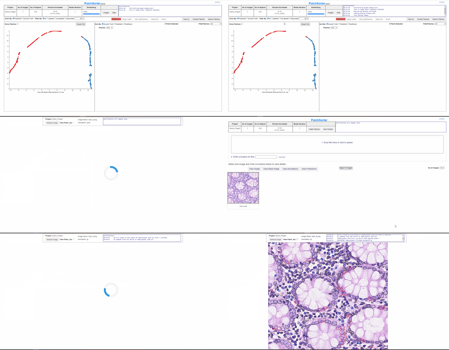
The image below shows, make patches successfully completed, and the next step is View Embed which directs user to Embedding Page.

6. Train DL, Embed Patches

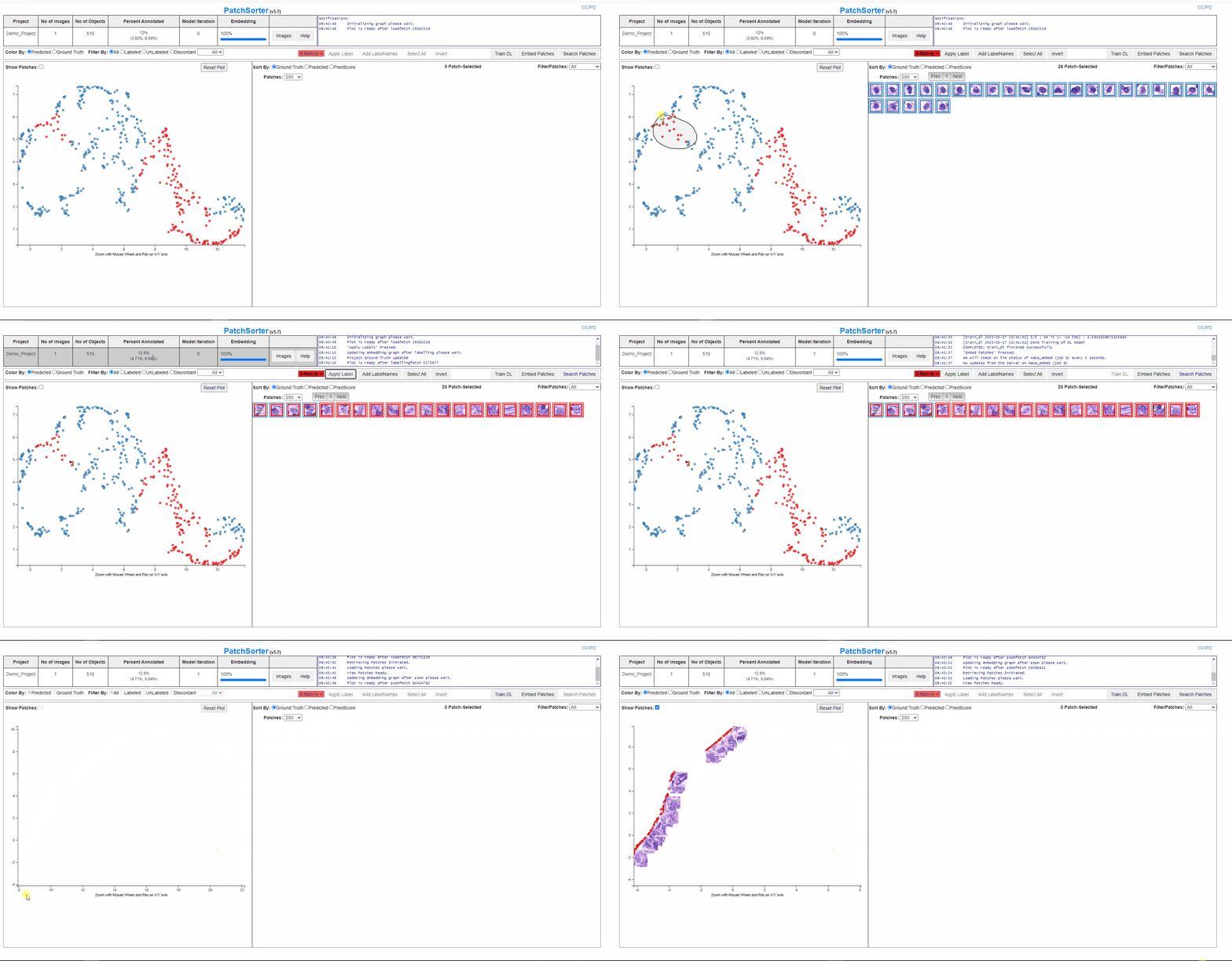
The image below shows, training DL successfully completed, and the next step is Embed Patches

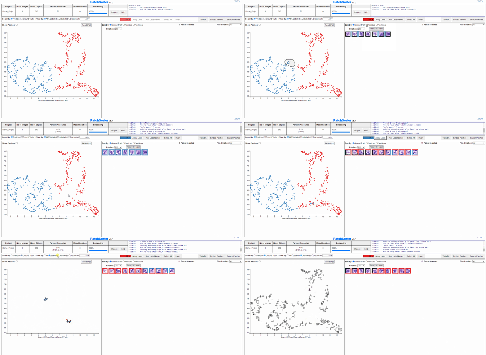
After the patches are embedded, a 2D scatter plot with all the patches represented as dot will be presented to the user. The patches will be clustered based on unsupervised Deep Learning Model and with further labelling , re training and embedding they will be separated into homogenous clusters.

7. Show Patches

User can click on Show Patches to check the distribution of the patches on the plot.

8. Labelling

On lasso over the plot points, the patches are loaded in the grid form.

Each patch will be shown with two colored border. Outer border indicates the predicted class and inner border is the ground truth, on unlabelled objects ground truth will be shown in black.

Once labelled it will change to the color of the class. The below image shows the process of labelling in brief.

Once some labelling is done, user will see an update in the labelling percentage, shown in screen below in green bubble.

And user could train the DL model and re-embed to see the clusters getting more organized homogenously.

9. Re-Train and Embed

The screen below is showing process of re-training and embedding. And the plot will get refreshed with the clusters seperated better and would be effective for a faster labelling.

10. View Predictions and Annotations

• Viewing the DL learning model predicted cell/object labels overlayed on the image.
• Viewing the annotated cell/object labels (labels that user assigned) overlayed on the image. Black color here would depict unlabeled data. These features help the user to view the labels with a better context and has an option to fine tune the labelling and update them back in the system.

The overlay mask and image also get saved in the projects folder in PatchSorter directory.